Section 5.1. Statistical Process Control
5.1. Statistical Process ControlThis chapter's example is a check processing operation. The number of checks varies by day of the week as does the amount of money deposited. These are measures of quantity and can be forecasted and monitored using techniques in Chapter 3. But quality is as important as quantity. If something is going wrong in the operation (e.g., if payments are being misapplied, or check numbers are being recorded incorrectly), we need to know. 5.1.1. Choosing MetricsWhen monitoring a manufacturing process we can measure the diameter of a bolt, the weight of a bottle of shampoo, or the percent of electrical components failing a test. These are things that do not vary by day of the week, and a significant change in any of them can mean trouble. In our check processing operation we need to use metrics that behave this way. First, we consider potential problem areas. Checks received for payment need to be processed quickly, so we measure the average age of the checks. Customers are supposed to send a remittance slip with their check, and we will measure the percentage of payments received that contain only a check and the average number of pages of remittance information per check. Money is important, so we measure both the average check amount and the average amount per remittance page. Finally, we need to monitor the accuracy of our data capture process. For this we look at the percentage of checks that have a valid invoice number, the average number of digits in the check number, and the average number of digits in the check amount. If any of these metrics shows a significant change we need to find the reason. Avoiding metrics based on volume or day of the week keeps the focus on quality. This concept can be applied to almost any operation. In a call center you might look at average talk time, percentage of calls abandoned, and percentage of calls transferred. In an invoicing area it could be average value, average lines, and product mix. 5.1.2. X and S ChartsThe process, like forecasting, is simply predicting what each metric should be, knowing how accurate the prediction is, and using this to set control limits for each metric. The prediction is the recent average. We don't consider lag since these metrics are not cyclic. We don't correct for the trend. If there is a trend, we want to know. We are looking for trends. We use two kinds of metrics. First is the average. In the example we look at the average number of pages per check. Second is the standard deviation. For some metrics we need to know if the amount of variation is changing. With number of pages per check, the average could be steady, yet we could be getting more really high and low page counts. Results are displayed on a chart like the one in Figure 5-1. Figure 5-1. Statistical Process Control chart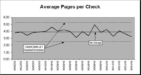 Charts dealing with averages are called X charts . Those dealing with standard deviation are called S charts . Years ago there were also charts that looked at the range (the difference between the highest and lowest measurement). They were called R charts , and were used because the calculations are simpler. Finding standard deviations by hand for hours every day is not as much fun as you might think. Today the distinction between X and S charts doesn't mean much. The terminology evolved before PCs and Excel. Statistical Process Control was a complex and labor intensive proposition. The metrics had to be manually collected and the calculations done by hand. Today you can probably collect all your metrics from automated sources and Excel takes care of the calculations. The control limits are usually set three standard deviations from the average. This means that 99.7 percent of the time the metric will be within the control limits if there is not a problem. This also means that three times in every thousand tests there is a false positive. Of course, you don't have to use three standard deviations. Three is commonly used because it gives good results and because that's what everyone else uses. But you can use a different number. The number of standard deviations used to set the control limits is called the sigma . It is a trade off. A low sigma is good at detecting problems, but it is also good at producing false positives. A high sigma means less work tracking down false alarms but a better chance of missing something important. We assume the metrics are normally distributed. In the real world few things really are, but it is easier to assume that they are normal than it is to figure out what is actually going on. There are times, however, when a different distribution gives better results. The application will let the user choose to use either a normal or log normal distribution . In a log normal distribution, the measures are skewed to the high end of the range. Using a log normal distribution to set the limits makes the application more sensitive to drops in the metric. It improves detection of skipped digit problems. This can be helpful in monitoring keying or OCR operations, for example. |
EAN: 2147483647
Pages: 101