3 Propagation aspects

The various types of attenuation to be considered when deploying a free-space optical communication network are geometrical attenuation, atmospheric attenuation, scintillation and optical mispointing.

3.1 Geometrical attenuation

The beam emitted by the transmitter being diverging (1 “3 mrad), the receiving cell will collect only some of the emitted energy. The following relation gives the geometrical attenuation:

where:

S _capture : Receiver capture surface (0,005 m ² , 0.025 m ² for example),
: Beam divergence ,
d: Transmitter-receiver distance.

3.2 Atmospheric attenuation

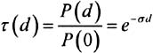
Atmospheric attenuation results from an additive effect of absorption and dispersion of the infrared light by aerosols and gas molecules present in the atmosphere. Transmittance in function of the distance is given by BEER relation:

where:

(d): Transmittance at distance d of the transmitter,
P(d): Power of the signal at a distance d of the transmitter,
P(0): Emitted power,
ƒ : Specific attenuation or extinction coefficient per unit of length.

Attenuation is connected to transmittance by the following expression:

The extinction coefficient ƒ is the sum of four terms:

where:

± _m is the molecular absorption coefficient (N2, O2, H2, HO, CO2, O3,..),
± _n is the absorption coefficient by the aerosols (small solid or liquid particles present in the atmosphere (ice, dust, smoke etc)
² _m is the Rayleigh scattering coefficient resulting from the interaction of the wave with particles of size smaller than the wavelength,
² _N is the Mie scattering coefficient. It appears when particles are of the same order of magnitude as the transmitted wavelength.

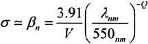
Absorption dominates in the infrared while scattering dominates in the visible and ultraviolet band . Being given the low values of molecular and aerosol absorption coefficients as well as Rayleigh scattering coefficient, the extinction coefficient can be written by the following relation:

where:

V is the visibility in km
» is the wavelength (nm)
Q is the size distribution of the diffusing particles
- = 1,6 for strong visibility (V>50 km),
- = 1,3 for average visibility (6<V<50 km),
- = 0,585 V ^1/3 for low visibility (V<6 km).

The visibility is a concept defined for meteorology needs to characterise the atmospheric transparency and estimated by a human observer. It is given by the atmospheric optical range and measured using a transmissometer or a diffusiometer.

3.3 Cloud attenuation

When the air cools beyond its saturation point, the water vapor condenses to form water droplets or ice crystal if the temperature is very low. Generally , the water particles thus formed have small sizes (<100 ¼ m), but their concentration can be important (a few hundreds per cm ³ ). The existence of the clouds is strongly related to the climate of the area considered. Cold moderate areas generally have a minimal cloud cover in summer whereas continuous rainfall is maximum. In the Mediterranean, the reverse is observed .

Presence of clouds is characterised by a nebulosity index which indicates the fraction of the sky covered and it is expressed in 1/10ths of percentage. The effects of multiple diffusion are important when a light beam crosses the cloud. The diffusion, in addition, involves a time and frequency scattering as well as a depolarisation.

3.4 Fog and haze attenuation

Fog and haze consist of very small water droplets (<100 ¼ m) suspended in the air. It is formed by a process of condensation close to the ground following radiative cooling of the ground ( especially at night) or to air movement on cold ground (advection fog or haze). To distinguish haze from fog, it is generally admitted that the visibility is higher than 1000 m in the presence of haze while it is lower than 1000 m in the presence of fog.

An excellent correlation was found between attenuation due to fog and liquid water concentration. The following relations for the attenuation coefficient were obtained at 0,63 ¼ m and 10,6 ¼ m [VASSEUR, 1997]:

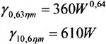
where W is the liquid water concentration (g/m ³ ).

The liquid water concentration in the fog is typically equal to approximately 0,05 g/m ³ for a moderate fog (visibility of about 300 m) and to 0,5 g/m ³ for a thick fog (visibility of about 50 m) [UIT-R P. 840 “3].

Weather measurements taken in Belgium in 16 stations during about twenty years provide indications on its maximum ( worse case) and median (not exceeded in 50% of the cases) annual frequency.

Table 18.2 gives the fog annual frequency [BODEUX, 1977].

Table 18.2: Annual frequency of fog
	Median frequency	Maximum frequency
Light, moderate or thick fog (V<1000 m)	0,055%	0,14%
Moderate or thick fog (V<500 m)	0,035%	0,11%
Thick fog (V<200 m)	0,020%	0,08%

3.5 Attenuation due to precipitation

The rain is formed from the water vapor contained in the atmosphere. It consists of water drops whose form and number are variable in time and space.

Attenuation due to rain is due primarily to the scattering phenomenon as in the case of aerosols. In infrared the wavelength is very much smaller than the raindrops' diameters. The value of the standardised cross section, Q _d remains equal to 2 whatever the wavelength.

The expression of the rain scattering coefficient is:

where R and dN(r) are respectively given in cm and in number/cm ⁴ .

When the size of the irregularities due to precipitations becomes important compared to the wavelength, the wave is attenuated by reflection and refraction. Attenuation, independent of the wavelength, is a function of the precipitation intensity R (in mm/h) according to the following relation:

where R is the rain intensity measured in mm/ hour .

Rain intensity is the fundamental parameter being used to locally describe the rain. Its measurement is carried out either directly on the ground by means of pluviometers or comparable apparatuses or in an indirect way by means of weather radar. The latter is particularly well adapted to the analysis of the rain structure. The relation given by Carbonneau et al.. [CARBONNEAU, 1998] is slightly different, attenuation values being much higher:

3.6 Other hydrometeors (snow, hail, etc)

Many other hydrometeors are present in nature. They are mixtures of ice, air and/or liquid water. Among these mixtures, snow is one of most complex. Snow generally falls in the form of flakes which are crystal aggregates of ice. The flakes can reach diameters of 15 mm. Although they do not have a defined form, one compares them to spheres and one classifies them by their water content after fusion.

Attenuation due to snow is strongly related to its humidity or density. Analysis of the experimental data [VASSEUR, 1997] makes it possible to release the following results:

For low humidity snow fall (dry snow), attenuation can reach 20 dB/km in the visible and 40 dB/km in infrared.
For wet snow falls, attenuation varies from 4 to 8 dB/km as well in the visible as in infrared.
Hail can be regarded as ice containing air bubbles . They are the largest observable hydrometeors (up to 8 cm in diameter).

3.7 Refraction and scintillation

Under the influence of thermal turbulence within the propagation medium the formation of random, variable size (10 cm-1 km) and of different temperature cells occur. These various cells have different refraction indexes thus causing scattering, multiple paths, arrival angle variations: the signal received quickly fluctuates at frequencies ranging between 0,01 and 200 Hz. The wave front varies in a similar way causing focusing and defocusing of the beam. Such signal fluctuations are called scintillations . Scintillation amplitude and frequency depend on the cell size compared to beam diameter. When heterogeneities are large compared with the beam cross section, it is deviated, when they are small, the beam is widened.

The tropospheric flicker effect is generally studied starting from the logarithm of the amplitude [dB] of the observed signal ("log-amplitude"), defined as the ratio in decibels of its instantaneous amplitude and its average value. Intensity and speed of the fluctuations (frequency of scintillations) increase with the wave frequency. For a plane wave, a weak turbulence and a specific receiver, the scintillation variance ƒ . ² [dB ² ] can be expressed by the following relation:

where:

k [m ^{ˆ’ 1} ] is the number of waves (2 / » ),
L [m] is the link length,
C _n ² [m ^{ˆ’ 2/3} ] is the structural parameter of the refraction index representing the turbulence intensity.

Scintillation peak-to-peak amplitude is equal to 4 ƒ and attenuation related to scintillation is equal to 2 ƒ . For strong turbulence, one observes a saturation of the variance given by the relation above [BATAILLE, 1992]. One will note that C _n ² parameter does not have the same value at millimeter and optical wavelengths [VASSEUR, 1997]. Millimeter waves are especially sensitive to humidity fluctuations while in optics, refraction index is a primarily function of the temperature (the water vapor contribution is negligible). One obtains in millimeter waves a value of C _n ² of about 10 ^{ˆ’ 13} m ^{ˆ’ 2/3} which is an average turbulence (in general in millimeter range we have 10 ^{ˆ’ 14} < C _n ² <10 ^{ˆ’ 12} ) and in optical a value of C _n ² about 2x10 ^{ˆ’ 15} m ^{ˆ’ 2/3} which is a light turbulence (in general in optics we have 10 ^{ˆ’ 16} < C _n ² <10 ^{ˆ’ 13} ), [BATAILLE, 1992].

3.8 Optical misalignment

Being given the equipment characteristic (low divergence of the laser beam), very precise alignment is necessary. The alignment of the transmitter and the receiver characterises optical link coupling. This one can be disturbed following mechanical vibrations.