99.

[Top] [Next] [Prev]

9.3 State Assignment

The number of gates needed to implement a sequential logic network depends strongly on how we assign encoded Boolean values to symbolic states. Unfortunately, the only way to obtain the best possible assignment is to try every choice for the encoding, an extremely large number for real state machines. For example, a four-state finite state machine, such as the traffic light controller of the last chapter, has 4! (4 factorial) = 4 * 3 * 2 * 1 = 24 different encodings (see Figure 9.19).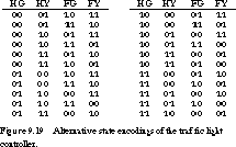

9.3.1 Traffic Light Controller

To illustrate the impact of state encoding on the next-state and output logic, let's use the symbolic state transition table for the traffic light controller, shown in Figure 9.20.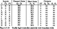

The input combinations that cause the state transitions are shown at the left of the table. The symbolic state names HG, HY, FG, FY represent the states highway green/farmroad red, highway yellow/farmroad red, highway red/farmroad green, and highway red/farmroad yellow. We have already encoded the traffic light outputs: 00 = Green, 01 = Yellow, and 10 = Red.

We can use espresso to examine the alternative state assignments rapidly.

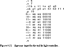
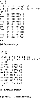
Figure 9.21 shows the generic truth table description that is input to espresso. We simply replace the symbolic state names HG, HY, FG, and FY with a particular encoding. Before we do a state assignment and two-level minimization, the finite state machine requires 10 unique product terms (one for each row of Figure 9.21).

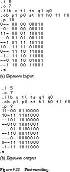
Figure 9.22 and Figure 9.22 show the results of espresso runs with the state assignments HG = 00, HY = 01, FG = 11, FY = 10 and HG = 00, HY = 10, FG = 01, FY = 11 respectively. A cursory glance shows that the second encoding uses fewer product terms, eight versus nine, and fewer literals, 21 versus 26.

Comparison of the Two Encodings Let's look at the relative complexity of the two implementations. The logic equations implied by the two alternative encodings are the following.

First encoding:

With conventional gate logic, the encoding requires 3 five-input gates, 2 four-input gates, 6 three-input gates, and 2 two-input gates, a total of 13 gates. We assume that variables and their complements are available to the network.

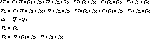
Second encoding:

This encoding requires 2 four-input gates, 8 three-input gates, and 3 two-input gates, for a total of 13 gates. This implementation uses the same number of gates, but it makes more extensive use of gates with smaller fan-ins. This reduces overall wiring and is one reason why it is often more useful to count literals than gates in comparing circuit -complexity.

In the next two subsections, we present methods for finding good state encodings. These are suitable for pencil and paper, as well as computer-aided design tools.

9.3.2 Pencil-and-Paper Methods

Without computer-aided design tools, there is little you can do to generate a good encoding. Hand enumeration using trial and error becomes tedious even for a relatively small number of states. An n-state finite state machine has n! different encodings. And this is only the lower bound. If the state is not densely encoded in the fewest number of bits, even more encodings are possible.

To make the problem more tractable when you must use hand methods, designers have developed a collection of heuristic "guidelines." These try to reduce the distance in Boolean n-space between related states. For example, if state Y is reached by a transition from state X, then the encodings should differ by as few bits as possible. The next-state logic will be minimized if you follow such guidelines. We examine them in this section.

State Maps State maps, similar in concept to K-maps, provide a means of observing adjacencies in state assignments. The squares of the state map are indexed by the binary values of state bits; the state given that encoding is placed in the map square. Obviously the technique is limited to situations in which a K-map can be used, that is, up to six -variables.

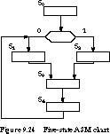
Figure 9.24 presents an ASM chart for a five-state finite state machine. Figure 9.25 gives two alternative state assignments and their representations in state maps.

Minimum-Bit-Change Heuristic One heuristic strategy assigns states so that the number of bit changes for all state transitions is minimized. For example, the assignment of Figure 9.25(a) is not as good as the one in Figure 9.25(b) under this criterion:

Transition	First Assignment Bit Changes	Second Assignment Bit Changes
S0 to S1:	2	1
S0 to S2:	3	1
S1 to S3:	3	1
S2 to S3:	2	1
S3 to S4:	1	1
S4 to S1:	2	2

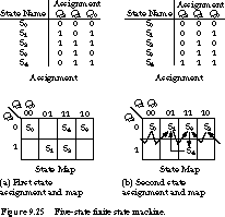
The first assignment leads to 13 different bit changes in the next-state function, the second only 7 bit changes.

We derived the first assignment completely at random and the second assignment with minimum transition distance in mind. Here is how we did it. We made the assignment for S0 first. Because of the way reset logic works, it usually makes sense to assign all zeros to the starting state. We make assignments for S1 and S2 next, placing them next to S0 because they are targets of transitions out of the starting state.

Note how we used the edge adjacency of the state map. This is so we can place S3 between the assignments for S1 and S2, since it is the target of transitions from both of these states.

Finally, we place S4 adjacent to S3, since it is the destination of S3's only transition. It would be perfect if S4 could also be placed distance 1 from S0, but it is not possible to do this and satisfy the other desired adjacencies.

The resulting assignment exhibits only seven bit transitions. There may be many other assignments with the same number of bit transitions, and perhaps an assignment that needs even fewer.

The minimum-bit-change heuristic, although simple, is not likely to achieve the best assignment. For a finite state machine like the traffic light controller, cycling through its regular sequence of states, the minimum transition distance is obtained by a Gray code assignment: HG = 00, HY = 01, FG = 11, FY = 10. This was the first state assignment we tried in the previous subsection, and it was not as good as the second assignment, even though the latter did not involve a minimum number of bit changes.

Guidelines Based on Next State and Input/Outputs Although the criterion of minimum transition distance is simple, it suffers by not considering the input and output values in determining the next state. A second set of heuristic guidelines makes an effort to consider this in the assignment of states:

Highest priority: States with the same next state for a given input transition should be given adjacent assignments in the state map.

Medium priority: Next states of the same state should be given adjacent assignments in the state map. Lowest priority: States with the same output for a given input should be given adjacent assignments in the state map.

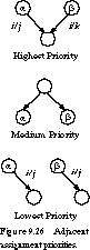
The guidelines, illustrated in Figure 9.26 for the candidate states a and b, are ranked from highest to lowest priority. The first two rules attempt to group together ones in the next-state maps, while the third rule performs a similar grouping function for the output maps. We do a state assignment by listing all state adjacencies implied by the guidelines, satisfying as many of these as possible.

Example Applying the Guidelines Consider the state transition table of Figure 9.13 for the 3-bit sequence detector. The corresponding state diagram is shown in Figure 9.27.

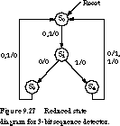
Let's apply the state assignment guidelines to this state diagram.The highest-priority constraint for adjacent assignment applies to states that share a common next state on the same input. In this case, states S3' and S4' both have S0 as their next state. No other states share a common next state.

The medium-priority assignment is for states that have a common ancestor state. Again, S3' and S4' are the only states that fit this -description.

The lowest-priority assignments are made for states that have the same output behavior for a given input. S0, S1', and S3' all output 0 when the input is 0. Similarly, S0, S1', S3', and S4' output 0 when the input is 1.

The constraints on the assignments can be summarized as follows:

Highest priority: (S3', S4');

Medium priority: (S3', S4');

Lowest priority: 0/0: (S0, S1', S3');
1/0: (S0, S1', S3', S4');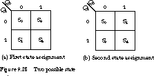

Since the finite state machine has four states, we can make the assignment onto two state bits. In general, it is a good idea to assign the reset state to state map square 0. Figure 9.28 shows two possible assignments. Both assign S0 to 00 and place S3' and S4' adjacent to each other.

Example Applying the Guidelines in a More Complicated Case As another example, let's consider the more complicated state diagram of the 4-bit string recognizer of Figure 9.7. Applying the guidelines yields the following set of assignment constraints:

Highest priority: (S3', S4'), (S7', S10');

Medium priority: (S1, S2), 2 ¥ (S3', S4'), (S7', S10');

Lowest priority: 0/0: (S0, S1, S2, S3', S4', S7');
1/0: (S0, S1, S2, S3', S4', S7', S10');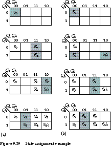

Figure 9.29 shows two alternative assignments that meet most of these constraints. We start with Figure 9.29(a) and first assign the reset state to the encoding for 0. Since (S3', S4') is both a high-priority and medium-priority adjacency, we make their assignments next. S3' is assigned 011 and S4' is assigned 111.

We assign (S7', S10') next because this pair also appears in the high- and medium-priority lists. We assign them the encodings 010 and 110, respectively. Besides giving them adjacent assignments, this places S7 near S0, S3', and S4', which satisfies some of the lower-priority -adjacencies.

The final adjacency is (S1, S2). We give them the assignments 001 and 101. This satisfies a medium-priority placement as well as the lowest--priority placements.

The second assignment is shown in Figure 9.29(b). We arrived at it by a similar line of reasoning, except that we assigned S7' and S10' the states 100 and 110. The second assignment does about as good a job as the first, satisfying all of the high- and medium-priority guidelines, as well as most of the lowest-priority ones.

Applying the Guidelines: Why They Work The state assignment guidelines attempt to maximize the adjacent groupings of 1's in the next-state and output functions. Let P2, P1, and P0 be the next-state functions, expressed in terms of the current state Q2, Q1, Q0 and the input X. To see how effective the guidelines were, let's compare the assignment of Figure 9.29(a) with a more naive assignment: S0 = 000, S1 = 001, S2 = 010, S3' = 011, S4' = 100, S7' = 101, S10' = 110.

Figure 9.30 compares the encoded next-state tables and K-maps for the two encodings. The 1's are nicely clustered in the next state K-maps for the assignment derived from the guidelines. We can implement P2 with three product terms and P1 and P2 with one each.

In the second assignment, the 1's are spread throughout the K-maps, since we made the assignment with no attempt to cluster the 1's usefully. In this implementation, the next-state functions P2, P1, and P0 each require three product terms, with a considerably larger number of literals overall.

9.3.3 One Hot Encodings

So far, our goal has been dense encodings: state encodings in as few bits as possible. An alternative approach introduces additional flip-flops, in the hope of reducing the next-state and output logic.

One form of this method is called one hot encoding. A machine with n states is encoded using exactly n flip-flops. Each state is represented by an n-bit binary code in which exactly 1 bit is asserted. This is the origin of the term "one hot."

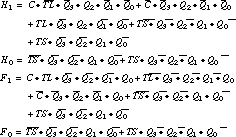
Let's consider the traffic light finite state machine described earlier in this section. The following would be a possible one hot encoding of the machine's state:

HG = 0001  HY = 0010  FG = 0100  FY = 1000 

The state is encoded in four flip-flops rather than two, and only 1 bit is asserted in each of the states.

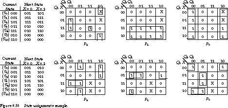
Figure 9.31 shows the espresso inputs and outputs for this encoding. It yields eight product terms, as good as the result of Figure 9.22. However, the logic is considerably more complex:

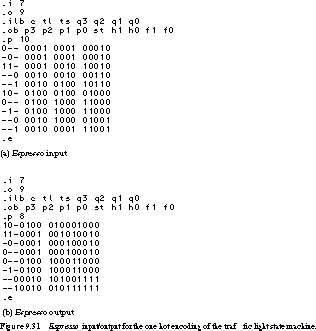
The product terms are all five and six variables, with two to five terms per output. This is rather complex for discrete logic but would not cause problems for a PLA-based design.

9.3.4 Computer Tools: Nova, Mustang, Jedi*

The previous subsections described various heuristic approaches for obtaining a good state encoding. None are guaranteed to obtain the best result. In this section, we examine three programs for computer-generated state assignments.

The state assignment guidelines of Section 9.3.2 place related states together in the state map, thereby clustering the 1's in those functions. However, we cannot evaluate an assignment fully without actually minimizing the functions. When it comes to hand techniques, this means the K-map method. If we have to use K-maps to minimize the functions for each possible assignment, we are not likely to examine very many of them!

Tools are available that follow the basic kinds of heuristics described above. Unlike hand methods, they are not limited to six state bits, they can generate many alternative assignments rapidly, and they can evaluate the derived assignments by invoking minimization tools like espresso or misII automatically. Three tools that provide this function are nova, for two-level logic implementations, and mustang and jedi, for multilevel logic. Jedi is somewhat more general; it can be used for -general-purpose symbolic encodings, such as outputs, as well as next states. We examine each of these programs in the following subsections.

Nova: State Assignment for Two-Level Implementation The inputs to nova are similar to the truth table format already described for espresso. The input file consists of the truth table entries for the finite state machine description. The latter are of the form:

inputs   current_state   next_state   outputs

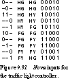
Figure 9.32 shows the format for our example traffic light controller. The states are symbolic; the inputs and outputs are binary encoded. It is important to separate each section with a space. We interpret the first line as "if input 1 (car sensor) is unasserted and the state is HG (highway green), then the next state is HG (highway green) and the outputs are 00010 (ST = 0, H1:H0 = 00 "green," F1:F0 = 10 "red").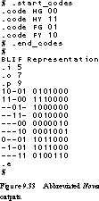

Figure 9.33 gives the abbreviated nova output associated with the state machine of Figure 9.32, assuming you have requested a "greedy" state assignment. The "codes" section shows the state assignment: HG = 00, HY = 11, FG = 01, and FY = 10. The espresso truth table is included in the output, indicating that it takes nine product terms to implement the state machine.

Intuitively, the state assignment algorithms used by nova are much like the assignment guidelines of Section 9.3.2. States that are mapped by some input into the same next state and that assert the same output are partitioned into groups. In the terminology of state assignment, these are called input constraints. Nova attempts to assign adjacent encodings within the smallest Boolean cube to states in the same group. A related concept is output constraints. States that are next states of a common predecessor state are given adjacent assignments.

Nova implements a wide range of state-encoding strategies, any of which you can select when you invoke the program:

• Greedy: makes its state assignment based on satisfying as many of the input constraints as it can. When using a greedy approach, nova looks only at new assignments that strictly improve on those it has already examined.
  
  
• Hybrid: also makes its state assignment based on satisfying the input constraints. However, nova will examine some assignments that start off looking worse, but may eventually yield a better assignment. This yields better assignments than the greedy strategy.
  
• I/O Hybrid: similar to hybrid, except it tries to satisfy input and output constraints. Its results are usually better than hybrid's.
  
  
• Exact: obtains the best encoding that satisfies the input constraints. Since the output constraints are not considered, this is still not the best possible encoding.
  
  
• Input Annealing: similar to hybrid, except it uses a more sophisticated method for improving the state assignment.
  
  
• One-Hot: uses a one-hot encoding. This rarely yields a minimum product term assignment, but it may dramatically reduce the complexity of the product terms (in other words, the literal count may be greatly reduced).
  
  
• Random: uses a randomly generated encoding. Nova will generate the specified number of random assignments. It will report on the best assignment it has found (the one requiring the smallest number of product terms).

For the traffic light controller, the various encoding algorithms yield the following assignments:

	HG	HY	FG	FY	Number of product terms	PLA Area
Greedy:	00	11	01	10	9	153
Hybrid:	00	11	10	01	9	153
Exact:	11	10	01	00	10	170
IO Hybrid:	00	01	11	10	9	153
I Annealing:	01	10	11	10	9	153
Random:	11	00	01	10	9	153

None of the assignments found by nova match the eight-product-term encoding we found in Figure 9.22. But we shouldn't despair just because the tool did not find the best possible assignment. The advantage of the computer-based tool is that it finds reasonable solutions rapidly. Thus you can examine a variety of encodings and choose the one that best reduces your implementation task.

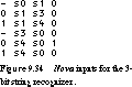
As another example, let's consider the 3-bit sequence recognizer of Figure 9.27. Its nova input file is shown in Figure 9.34. The state assignments found by nova are the following:

	S0	S1'	S3'	S4'	Number of product terms	PLA Area
Greedy:	00	01	11	10	4	36
Hybrid:	00	01	10	11	4	36
Exact:	00	01	10	11	4	36
IO Hybrid:	00	10	01	11	4	36
I Annealing:	00	01	11	10	4	36
Random:	00	11	10	01	4	36

Several of the assignments correspond to the ones found in Figure 9.28(a) and (b).

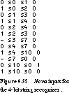
The last example is the 4-bit recognizer of Figure 9.7. The nova input file is given in Figure 9.35. Nova produced the following -assignments:

	S0	S1	S2	S3'	S4'	S7'	S10'	Number of product terms
Greedy:	100	110	010	011	111	000	001	7
Hybrid:	101	110	111	001	011	000	010	7
Exact:	101	110	111	001	011	000	010	7
IO Hybrid:	110	011	001	100	101	000	010	7
I Annealing:	100	101	001	111	110	000	010	6
Random:	011	100	101	110	111	000	001	7

None of these assignments match those derived in Figure 9.29, since S0 has not been assigned 000. Figure 9.36 shows that the adjacencies that were highly desirable based on the guidelines-that is, S3' adjacent to S4', S7' adjacent to S10', and S1 adjacent to S2-are satisfied by the input annealing assignment.

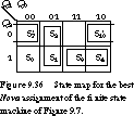
Mustang The minimum number of product terms is a good criterion if you are going to implement the logic in a two-level form, such as a PLA. This is what nova uses. Literal count is better if you plan to implement the logic in multiple levels. Mustang takes this approach. Its optimization criterion is to minimize the number of literals in the multilevel factored form of the next-state and output functions.

Mustang has an input format similar to that of nova. The only difference is that the number of inputs, outputs, and state bits must be explicitly declared with .i, .o, and .s directives. For example, the traffic light input file is shown in Figure 9.37.

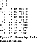
Mustang implements several alternative strategies for state assignment, specified by the user on the command line. These include:

• Random: chooses a random state encoding.
  
  
• Sequential: assigns the states binary codes in a sequential order.
  
  
• One-Hot: makes a one-hot state assignment.
  
  
• Fan-in: works on the input and fan-in of each state. Next states that are produced by the same inputs from similar sets of present states are given adjacent state assignments. The assignment is chosen to maximize the common subexpressions in the next-state function. This is much like the high-priority assignment guideline of Section 9.3.2.
  
  
• Fan-out: works on the output and fan-out of each state, without regard to inputs. Present states with the same outputs that produce similar sets of next states are given adjacent state assignments. Again, this maximizes the common subexpressions in the output and next-state functions. This approach works well for finite state machines with many outputs but few inputs. It is much like the medium- and low-priority assignment guidelines from Section 9.3.2.

Mustang derives the following assignments for the traffic light state machine:

	HG	HY	FG	FY	Number of product terms
Random:	01	10	11	00	9
Sequential:	01	10	11	00	9
Fan-in:	00	01	10	11	8
Fan-out:	10	11	00	01	8

The eight term encodings are actually better than any of those found by nova. To determine the multilevel implementation, you must invoke misII on the espresso file created by mustang.

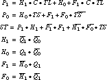
For example, the misII output for the fan-in encoding of the traffic light controller is the following:

For comparison with nova, mustang obtains the following encodings for the 3-bit string recognizer:

	S0	S1	S3'	S4'	Number of product terms
Random:	01	10	11	00	5
Sequential:	01	10	11	00	5
Fan-in:	10	11	00	01	4
Fan-out:	10	11	00	01	4

The number of product terms to implement an encoding is comparable to the number needed for the nova encodings. However, don't forget that the goal of mustang is to reduce literal count rather than product terms.

As a final example, let's look at the mustang encodings for the 4-bit recognizer:

	S0	S1	S2	S3'	S4'	S7'	S10'	Number of product terms
Random:	101	010	011	110	111	001	000	8
Sequential:	001	010	011	100	101	110	111	8
Fan-in:	100	010	011	000	001	101	110	8
Fan-out:	110	010	011	100	101	000	001	6

It is interesting that in all three cases, mustang obtained an encoding that is as good as any of the best encodings found by nova.

Jedi The final encoding program we shall examine is jedi. It is similar to mustang in that its goal is to obtain a good encoding for a multilevel implementation. It is more powerful than mustang because it can solve general encoding problems: jedi can find good encodings for the outputs as well as the states.

Like the other programs, jedi implements several alternative encoding strategies that can be selected on the command line. Besides random, one hot, and straightforward, the program supports input dom-i-nant, output dominant, modified output dominant, and input/output combination algorithms.

The jedi input format is similar to, but slightly different from, the mustang input format. We can illustrate this best with an example. Figure 9.38 shows the jedi input file for the traffic light controller. The present state and next states each count as a single input, even though they may be encoded by several bits. The .enum States line tells jedi that there are four states and that they should be encoded in 2 bits and then gives the state names. The .enum Colors line tells jedi that there are three output colors and that these should also be encoded in 2 bits. You should think of these as enumerated types. The .itype and .otype lines define the types of the inputs and outputs, respectively.

The encodings obtained from jedi for the traffic light controller are:

	HG	HY	FG	FY	Grn	Yel	Red	Number of product terms
Input:	00	10	11	01	11	01	00	9
Output:	00	01	11	10	10	11	01	9
Combination:	00	10	11	01	10	00	01	9
Output':	01	00	10	11	10	00	01	10

For the 3-bit string recognizer, the state assignments are:

	S0	S1	S3'	S4'	Number of product terms
Input:	01	00	11	10	4
Output:	11	01	00	10	4
Combination:	10	00	11	01	4
Output':	11	01	00	10	4

Finally, for the 4-bit string recognizer, they are:

	S0	S1	S2	S3'	S4'	S7'	S10'	Number of product terms
Input:	111	101	100	010	110	011	001	7
Output:	101	110	100	010	000	111	011	7
Combination:	100	011	111	110	010	000	101	7
Output':	001	100	101	010	011	000	111	6

Let's look at one head-to-head comparison between mustang and jedi. We will use the mustang encoding in which HG = 00, HY = 01, FG = 10, FY = 11, Green = 00, Yellow = 01, and Red = 10 and the jedi encoding in which HG = 00, HY = 01, FG = 11, FY = 10, Green = 10, Yellow = 11, and Red = 01. The first encoding used eight product terms in a two-level implementation; the second used nine.

The multilevel implementation for the mustang assignment was already shown in the mustang section. It requires 26 literals. The jedi multilevel implementation is

It has 27 literals. In terms of straight literal count, the mustang encoding is better. If we examine the wiring complexity, the mustang encoding is also slightly better.

[Top] [Next] [Prev]

---

This file last updated on 07/15/96 at 06:40:56.
[e-mail];