Showing and Hiding Options

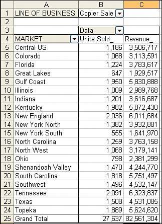
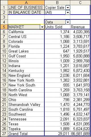
By their nature, pivot tables will summarize and show the data from all records in your dataset. There may, however, be situations when you want to inhibit certain data items from being included in your pivot table summary. In these situations, you can choose to hide a data item.

The Basics of Hiding an Item

When you hide a data item, you are not only preventing the data item from being shown on the report, you are also preventing it from being factored into the summary calculation.

Figure 5.1 shows a pivot table with Market in the row area. Two numeric fieldsUnits Sold and Revenueappear along the column area. Line of Business is in the page area and is currently set to Copier Sales.

Figure 5.1. This pivot table summarizes all copier sales, and it reports $86 million in sales.

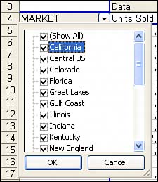
Note that the Market field contains a drop-down arrow on the right side of cell A4. If you select this drop-down, as shown in Figure 5.2, you will see a list of all the pivot items along the market dimension. By default, all the market items are selected.

Figure 5.2. The Market drop-down contains a list of all the markets. By default, all are selected.

To hide one market, you can uncheck the check box for that item. If your manager needs a report of all markets except California, simply uncheck California.

After you click OK to close the selection box, the pivot table instantly recalculates, leaving out the California market. As shown in Figure 5.3, the total copier sales drops by $4 million to $82 million without California.

Figure 5.3. After California is removed, the report recalculates without California's $4 million in sales.

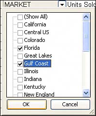
CAUTION

There is no outward sign that this report has been filtered to exclude California. Normally, you would expect Excel to change the arrow color of a filtered field to blue to indicate that some items are hidden. That functionality was not added to the pivot field arrows.

Showing All Items Again

You can just as quickly reinstate all hidden data items for a field with a few clicks. Select the drop-down arrow in the Market field and select the (Show All) selection. This will cause all unchecked items to reassume a checked state.

Showing or Hiding Most Items

In Excel 2002 and later, it is easy to produce a report that includes only two or three items along a dimension. If you need to produce a report of just Florida and the Gulf Coast, this will require only a few mouse clicks.

Select the Market drop-down. Unselect the (Show All) option, and all the markets will become unselected.

You can now select just Florida and Gulf Coast, as shown in Figure 5.4.

Figure 5.4. In Excel 2002 and later, it takes just three mouse clicks to unselect all markets and then to select two markets.

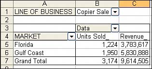
Figure 5.5 shows that Florida and the Gulf Coast accounted for $9.6 million of copier sales. This task is fairly easy in Excel 2002 and later.

Figure 5.5. This pivot table has all markets except two hidden.

NOTE

Excel 2000 does not offer the (Show All) option. This could present a significant problem if there were, for example, 200 customers and you needed to display only two of the customers. If you don't particularly feel like unchecking 198 items to get the view you need, an alternative solution would be to use the group method to create two or three groups of all the undesired markets. You could then easily uncheck these three groups. You will learn about the group method later in this chapter.

In Excel 97, you would have to double-click your field and then highlight the items to be hidden.

Hiding or Showing Items Without Data

By default, your pivot table will only show data items that have data. This inherent behavior may cause unintended problems for your data analysis. Look at Figure 5.6, which shows a pivot table with a date field in the page area. When the date field is set to (All), all 21 markets appear in the report.

Figure 5.6. A page field containing dates has been added to this pivot table.

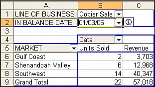
Select January 3 from the date page field, and the pivot report redraws to show only the three markets with copier sales on that day. Figure 5.7 shows that these markets happened to be Gulf Coast, Shenandoah Valley, and Southwest.

Figure 5.7. By default, a pivot table will hide the markets with no data for this combination of page field selections.

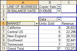
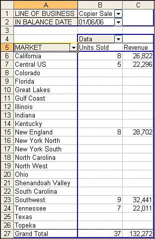
Select a different date from the date page field. The report will redraw to include the markets with sales on that day. Figure 5.8 shows that on January 6, there were five markets with copier sales.

Figure 5.8. Change the date in the page field, and a different set of markets will appear.

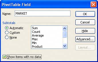
The behavior of displaying only items with data makes for a very concise report, but it could be annoying if you later wish to compare snapshots of several days. In that case, you might wish that Excel would show you all 21 markets every time. To prevent Excel from hiding pivot items without data, double-click the Market field to display the PivotTable Field dialog box, as shown in Figure 5.9. In the lower-left corner, choose Show Items with No Data.

Figure 5.9. Double-click the Market field to display this dialog box. Choose the box in the lower-left corner to force all markets to display.

After you choose the Show Items with No Data option, all the markets will appear, regardless of whether they had sales that day, as shown in Figure 5.10.

Figure 5.10. It would be easier to compare a snapshot of this report with other days after all days contain the same list of markets.

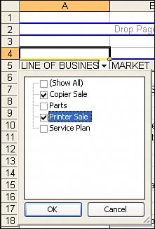
Hiding or Showing Items in a Page Field

A page field typically includes either (All) or one pivot item. If you select the Line of Business drop-down, you can either select one single line of business or select the (All) option to see all lines of business. There does not appear to be a way to create a report with the total of copier sales and printer sales.

The solution is to drag the Line of Business field into either the row or the column area of your report. After it is there, use the Line of Business drop-down to select only printer and copier sales, as shown in Figure 5.11.

Figure 5.11. Temporarily drag the page field to the row area and then select the desired product lines.

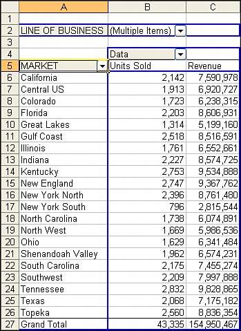
After choosing two items, drag the Line of Business field back to the page area of the report. Magically, a new option called (Multiple Items) will be selected in the page field, as shown in Figure 5.12.

Figure 5.12. Drag the Line of Business field back to the page area, and the pivot table remembers the two lines selected in the previous step.

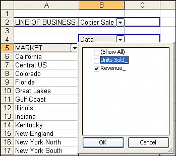
CAUTION

After using this technique, you have no way to add hidden items back to the page field. You will have to drag the page field back to the row or column area to show the hidden items.

Showing or Hiding Items in a Data Field

In Excel 2000 and later, pivot reports with multiple fields in the data area of the report will include a gray data field with a drop-down. To remove the Units Sold field from the data area, you can use one of two methods. You can uncheck the item from the Data drop-down, as shown in Figure 5.13.

Figure 5.13. After you have multiple data fields, there is no way to drag one of the data fields from the report. You can use the Data drop-down to remove the field.

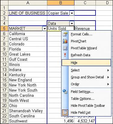
Alternatively, you can right-click the Units heading and choose Hide, as shown in Figure 5.14.

Figure 5.14. Alternatively, you can remove a data field by right-clicking the field name and choosing Hide.