Routing
| A routing engine calculates the optimum path between an origin and destination, subject to certain criteria. Common criteria include "use freeways," "avoid freeways," or "fewest turns." The most common algorithm for calculating routes is based on the A* (pronounced A-star ) algorithm developed in the artificial intelligence (AI) community. The algorithm works by extending each known possible path to the destination by adding an intelligent guess (a heuristic estimate) and computing the total cost of the real traversed path plus the heuristic estimate. Understanding routing requires understanding the basics of problem solving using AI techniques. The effectiveness of a combinatorial and problem-solving technology is significantly dependent on the way that the software represents the problem's states, goals, and conditions. Typically, these problems are represented using graphs and trees. The most common routing problems are referred to as shortest path, traveling salesman, multiple traveling salesman , single depot “multiple vehicle, and multiple vehicle “multiple depot routing. The simplest and most often used is the shortest path between two points, which we explore first. Routing Problems DefinedShortest Path ProblemFigure 4.14 shows a graphical example of the shortest path problem. Figure 4.14. A Simple Road Network with Each Node Numbered. The Dotted Line, Indicating a Straight Path Between Current Location and Destination, Is a Common Heuristic Used to Complete the Path. 2002 Kivera, Inc. The A* Algorithm in ActionSpatial analysis software vendors often use a two-sided A* algorithm for routes, expanding from both origin and destination simultaneously . For simplicity, because the principles remain the same, a single-sided example is examined here. Starting at the origin, node 23, the algorithm explores four possible paths. At the end of each link the path to the destination is completed with the addition of the heuristic path. Thus, the first four paths to try would be, in no particular order:
These are then sorted by cost (time):
Next , the algorithm expands from the fastest path so far:
Add these paths to the total number of paths traversed so far and order again from fastest to slowest:
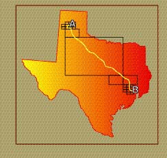
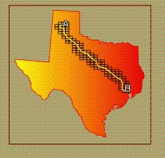
As the potential paths grow, there will be opportunities to select roads belonging to faster arterial levels. At node 40, for example, the algorithm will always "jump" to the faster arterial level. This jump to a higher arterial level often results in a jump to a larger cell size as well. These cells cover a greater area and have fewer road segments per unit area. As seen in Figure 4.15, jumping up to cells that cover more area results in having to read in fewer cells and consequently faster routing. Figure 4.16 shows the many more cells , each with a higher road density and therefore more data to read that have to be examined if there is no opportunity to jump to higher levels. Figure 4.15. Jumping to Cells That Cover a Larger Area Results in a Routing Algorithm That Requires Fewer Cells and Operates Faster. 2002 Kivera, Inc. Figure 4.16. A Routing Algorithm That Is Constrained to One Level of Cells Must Read in Many More Cells. 2002 Kivera, Inc. It is common to use the A* algorithm for routing. However, this does not mean that all implementations of the A* algorithm are created equal. About 10 independent parameters serve as input into the algorithm, and even small changes in these parameters result in large changes in what route is taken. Traveling Salesman ProblemThe traveling salesman problem is the least time-consuming path that passes through each node of a connected network once. A simple example is shown in Figure 4.17, where a salesman must visit each of five cities, labeled A through E. There is a road between every pair of cities, with the distance given next to the road. From point A, the objective is to visit each city once and then return to A. Figure 4.17. Traveling Salesman Map. The simple method to solve this problem involves creating a search tree that explores possible paths until the search criteria have been met (see Figure 4.18). Figure 4.18. Traveling Salesman Search Tree. Multiple Traveling Salesman ProblemThis problem is the same as the single traveling salesman problem, except it involves multiple salesmen (vehicles) leaving from and returning to the same location. Single Depot “Multiple Vehicle Node RoutingThis problem involves vehicle routing, providing a solution for a set of delivery routes for vehicles stored at a central depot. Multiple Depot “Multiple Vehicle Node RoutingThis problem requires a solution similar to the single depot “multiple vehicle problem, except with multiple depots. Vehicles must leave from and return to the same depot. What Impacts Route Calculation Performance?A route engine typically considers six segment attributes in calculating a route:
Preprocessing and reducing the number of attributes the route engine has to consider both improve route performance. |
EAN: 2147483647
Pages: 150