13. | FrameMaker 6: Beyond the Basics

Preparing a Form's Functionality

The form now looks good. The next step is to build the functionality for printing the report. You need a way to change between the different row views, and you need a way to hide any unwanted columns. Excel can store different views of a worksheet that you specify, which you can then show later as needed. If you build some views into the worksheet, creating a macro to change between views will be easy.

Create Custom Views on a Worksheet

A custom view allows you to hide rows or columns on a worksheet and then give that view a name so that you can retrieve it easily. You need to create three views. The first view shows all the rows and columns. That one is easy to create. The second view shows only the total rows. The third view shows only the detail rows. Hiding the rows can be a tedious process. Fortunately, you need to hide them only once. You can also use Excel's Go To Special command to help select the rows faster.

Activate Excel. From the View menu, click the Custom Views command.
In the Custom Views dialog box, click the Add button, type All as the name for the new view, clear the Print Settings check box, leave the Hidden Rows, Columns And Filter Settings check box selected, and then click OK.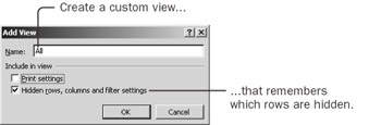

You just created the first view, the one with all rows and columns displayed. You now need to create the Summary view, showing only the total rows. That means that you need to hide the detail rows. You notice that only the detail rows have labels in column B.
Select column B. From the Edit menu, click Go To and then click Special. Select the Constants option, and click OK.

Only the cells in the detail rows are still selected.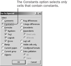
Hide the selected rows. (From the Format menu, click Row, and then click Hide.)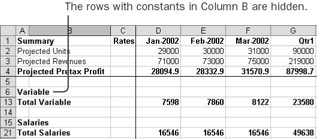

The only remaining rows that you want to hide all have blank cells in column D. Does that give you any ideas?
Select column D. Click Edit, Go To, and Special. Select Blanks, and then click OK. Hide the selected rows as you did in step 4. This is the view for the managers.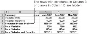
With only these total rows visible, create another view named Summary. (From the View menu, click Custom Views, click Add, type Summary, clear Print Settings, and then click OK.) Now you need to create the detail view. For the detail view, you want to hide all the summary rows. The rows you want to hide have labels in the range A4:A54.
Show the All custom view to unhide all the rows. (From the View menu, click Custom Views, and with All selected, click OK.) Select the range A4:A54, use Go To Special to select the cells with constants, and then hide the rows. Select column D, and hide all the rows with blank cells.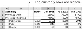
With these detail rows visible, create a new view named Detail, again clearing the Print Settings option.
Save the workbook, and try showing each of the three views. Finish with the All view.

Creating the views is bothersome, but you have to do it only once. Once the views are created, making a macro to switch between views is easy.

Create a Macro to Switch Views

Start recording a macro named ShowView. Show the Summary view, turn off the recorder, and look at the macro. It should look like this:
```
Sub ShowView()     ActiveWorkbook.CustomViews("Summary").Show End Sub
```
A Workbook object has a collection named CustomViews. You use the name of the view to retrieve a CustomView item from the collection. A CustomView object has a Show method. To switch between views, all you need to do is substitute the name of the view in parentheses. And rather than create three separate macros, you can pass the name of the view as an argument.
Type ViewName between the parentheses after ShowView, and then replace "Summary" (quotation marks and all), with ViewName. The revised macro should look like this:
```
Sub ShowView(ViewName)     ActiveWorkbook.CustomViews(ViewName).Show End Sub
```
Next you'll test the macro and its argument using the Immediate window.
Press Ctrl+G to display the Immediate window.
Type ShowView "Detail" and press the Enter key.

The worksheet should change to show the detailed view.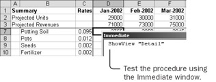
Type ShowView "All" and press the Enter key. Then type ShowView "Summary" and press the Enter key again. The macro works with all three arguments.
Close the Immediate window, and save the workbook.

You now have the functionality to show different views. Creating the views might not have been fun, but it certainly made writing the macro a lot easier. Also, if you decide to adjust a view (say, to include blank lines), you don't need to change the macro.

At this point, you need to create the functionality to hide columns containing dates earlier than the desired starting month.

Dynamically Hide Columns

You don't want to create custom views to change the columns because you'd need to create 36 different custom views-one for each month times the three different row settings. You need to change the columns dynamically, based on the choices in the dialog box. If you're going to hide columns, you'll start with column C and end with an arbitrary month specified. One good way to find the month is to use Excel's Find method.

In Excel, select all of row 1 and then start recording a macro named HideMonths.
From the Edit menu, click the Find command and then click the Options button to expand the dialog box. Type 5/1/2002 in the Find What box, select the Match Entire Cell Contents check box, and make sure the Look In drop-down list box says Formulas.

Important
If your system uses a date format other than mm/dd/yyyy (the default United States date format), you'll need to experiment to find the date format that works for you.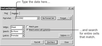

By searching for the formula, you look for the underlying date in the cell. The underlying date uses the system date format, regardless of how the cell happens to be formatted. By searching only entire cells, you make sure that 1/1/2002, for example, will find only January (1/1/2002), and not November (11/1/2002), which differs only by having an extra digit at the beginning.
Click Find Next, close the Find dialog box, stop the recorder, and then edit the HideMonths macro. Put a line continuation (a space, an underscore, and a new line) after every comma to make the statement readable. The macro should now look like this:
```
Sub HideMonths()     Selection.Find(What:="5/1/2002", _         After:=ActiveCell, _         LookIn:=xlFormulas, _         LookAt:=xlWhole, _         SearchOrder:=xlByRows, _         SearchDirection:=xlNext, _         MatchCase:=False, _         SearchFormat:=False).Activate End Sub
```
The macro searches the selection (in this case, row 1), starting with the active cell (in this case, cell A1), searches for the specified date, and activates the matching cell. You don't want the macro to change the selection, and you don't want the macro to activate the cell it finds. Rather, you want the macro to assign the found range to a variable so that you can refer to it.
Make these changes to the macro: Declare the variable myFind as a Range. Change Selection to Rows(1) and ActiveCell to Cells(1). Delete .Activate from the end of the Find statement, and add Set myFind = to the beginning.The revised macro looks like this:
```
Sub HideMonths()     Dim myFind as Range     Set myFind = Rows(1).Find(What:="5/1/2002", _         After:=Cells(1), _         LookIn:=xlFormulas, _         LookAt:=xlWhole, _         SearchOrder:=xlByRows, _         SearchDirection:=xlNext, _         MatchCase:=False, _         SearchFormat:=False) End Sub
```
If the Find method is successful, then myFind will contain a reference to the cell that contains the month. You want to hide all the columns from column C (the Rates column) to one column to the left of myFind.
Before the End Sub statement, insert this statement:
```
Range("C1",myFind.Offset(0,-1)).EntireColumn.Hidden = True
```
This selects a range starting with cell C1 and ending one cell to the left of the cell with the month name. It then hides the columns containing that range.

Save the workbook, and press F8 repeatedly to step through the macro. Watch as columns C through H disappear.

You'll be changing this subroutine to hide columns up to any date. You need some way of knowing whether or not the Find method finds a match. If the Find method does find a match, it assigns a reference to the variable. If it doesn't find a match, it assigns a special object reference, Nothing, to the variable. You can check to see whether the object is the same as Nothing. Because you're comparing object references and not values, you don't use an equal sign to do the comparison. Instead, you use a special object comparison word, Is.

Important

A variable that's declared as a variant contains the value Empty when nothing else is assigned to it. A variable that's declared as an object contains the reference Nothing when no other object reference is assigned to it. Empty means 'no value,' and Nothing means 'no object reference.' To see whether the variable myValue contains the Empty value, use the expression IsEmpty(myValue). To see whether the variable myObject contains a reference to Nothing, use the expression myObject Is Nothing.

Add the If and End If statements around the statement that hides the columns, resulting in this If structure:
```
If Not myFind Is Nothing Then     Range("C1", myFind.Offset(0, -1)) _         .EntireColumn.Hidden = True End If
```
If the Find method fails, it assigns Nothing to myFind, so the conditional expression is False and no columns are hidden.
Test the macro's ability to handle an error by changing the value for which the Find method searches, from 5/1/2002 to Dog. Then step through the macro and watch what happens when you get to the If structure. Hold the mouse pointer over the myFind variable and see that its value is Nothing.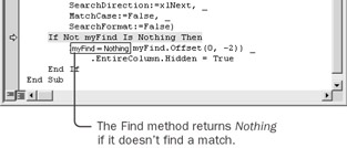

If you search for a date that's in row 1, myFind will hold a reference to the cell containing that date, and the macro will hide the months that precede it. If you search for anything else, myFind will hold a reference to Nothing, and the macro won't hide any columns.
Press F5 to end the macro.

The final step is to convert the date to an argument. Type StartMonth between the parentheses after HideMonths, and replace "5/1/2002"or "Dog" (including the quotation marks) with StartMonth. The revised (and finished) procedure should look like this:

Sub HideMonths(StartMonth )    Dim myFind As Range     Set myFind = Rows(1).Find(What:=StartMonth, _         After:=Cells(1), _         LookIn:=xlFormulas, _         LookAt:=xlWhole, _         SearchOrder:=xlByRows, _         SearchDirection:=xlNext, _         MatchCase:=False, _         SearchFormat:=False)     If Not myFind Is Nothing Then         Range("C1", myFind.Offset(0, -1)) _             .EntireColumn.Hidden _         = True      End If End Sub

Now test the macro. Press Ctrl+G to display the Immediate window. Enter ShowView "All" and then enter HideMonths "8/1/2002".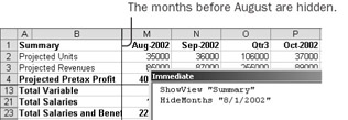
Close the Immediate window, and save the workbook.

You now have macros that can handle the functionality of the form by hiding appropriate rows and columns. It's now time to put the form and the functionality together.