Entering Values and Formulas into a Range

You may have situations where you want to create a macro that dynamically enters formulas into cells. First you should understand how references work in formulas in Excel, and then you can see how to create formulas in a macro.

See Also 

This section refers to standard Excel formula references. For information about using structured formulas in a table, see the section titled “Record a Macro to Manipulate a Table” in Chapter 5, “Explore Data Objects.”

Relative References

Most formulas perform arithmetic operations on values retrieved from other cells. Excel formulas use cell references to retrieve values from cells. Imagine, for example, a list of Retail prices and Wholesale costs.

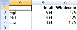
Suppose you want to add a column to the list that calculates the gross margin-the difference between the Retail price and the Wholesale cost-for each item. You would put the label Margin in cell D1 and then enter the first formula into cell D2. The formula subtracts the first Wholesale cost (cell C2) from the first Retail price (cell B2). So you would enter =B2-C2 into cell D2.

For each item in the High group, the gross margin is $2.75. Now you need to copy the formula to the other rows. The formula you typed into cell D2 refers explicitly to cells C2 and B2. When you copy the formula to cell D3, you want the formula to automatically adjust to refer to C3 and B3. Fortunately, when you copy the formulas, Excel adjusts the references because, by default, references are relative to the cell that contains the formula. (The Prices worksheet in the Chapter04 workbook contains these formulas.)

If the reference =C2 is found in cell D2, it really means “one cell to my left.” When you copy the formula to cell D3, it still means “one cell to my left,” but now that meaning is represented by the reference =C3.

Absolute References

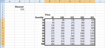
Sometimes you don’t want relative references. Imagine, for example, a worksheet that contains various quantities in column B and prices in row 3. (The Revenue worksheet in the Chapter04 workbook contains the prices and quantities.)

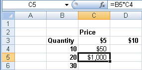
Suppose you want to add formulas to calculate the revenue for each combination. To calculate the first revenue value (cell C4), you need to multiply the first quantity (cell B4) by the first price (cell C3) . When you type = B4*C3 into cell C4, you get the correct answer: $50.

But if you copy that formula to cell C5, you get the ridiculous answer of $1000. That’s because the cell references are relative. In this version of the formula, you’re not really referring to cells B4 and C3; you’re referring to “one cell to my left” and “one cell above me.” When you put the formula into cell C5, “one cell above me” now refers to cell C4, not cell C3.

In the Revenue table, you want the Quantity cell references to adjust from row to row , and you want the Price cell references to adjust from column to column, but you always want to reference the Quantity from column B and the Price from row 3. The solution in the user interface is to put a dollar sign ($) in front of the B in the first Quantity reference ($B4), andin front of the 3 in the first Price reference (C$3). The formula that should go into cell C4 is =$B4*C$3. The dollar sign “anchors” that part of the formula, making it absolute. When you copy the formula to the rest of the range C4:E8, you get correct answers. (The RevenueFormulas worksheet in the Chapter04 workbook contains the correct formulas.)

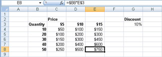
The relative portion of the formula changes with the row or column of the cell that contains the formula. The absolute portion remains fixed.

If you want to modify the formula so that it also takes into account the discount value from cell G3, you must make both the row and the column of the discount reference absolute. The correct formula would be =$B4*C$3*(1-$G$3). If you assign a name to a cell-for example, if you assign the name Discount to cell G3-then by default, usingthe name in the formula acts as a completely absolute reference. (The RevenueFormulas worksheet in the Chapter04 workbook contains these formulas.) Later in this chapter, you will create a macro that will fill the grid with the correct formula, regardless of where it is on the worksheet and how many rows or columns it has.

R1C1 Reference Style

As a default, Excel displays letters for column headings and numbers for row headings. Consequently, the default name for the upper-left cell in the worksheet is cell A1. Referring to cells by letter and number is called A1 reference style. In A1 reference style, however, cell references do not really say what they mean. For example, the reference =C4 says “cell C4,” but if it’s in a formula in cell E4, it really means “two cells to my left,” and if it’s in a formula in cell C5, it really means “one cell above me.” You don’t know what the reference really means until you know which cell contains the reference.

Excel has an alternate reference style that uses numbers for both column and row headings. In this alternate reference style, to refer to a cell you use the letter R plus the row number and C plus the column number. Consequently, the upper-left cell in the worksheet is cell R1C1. Referring to cells by numbers in both rows and columns is called R1C1 reference style. In R1C1 reference style, cell references really do say what they mean. Consequently, in macros, when VBA has to understand and use the formulas, itis usually convenient to use R1C1 reference style. When a human has to understand the formula, it is usually easier to use A1 reference style, which is why A1 reference style is the default.

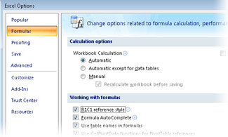
You can, however, change the user interface to use R1C1 reference style if you want totry it out. To turn on R1C1 reference style, click the Microsoft Office Button and then click Excel Options. On the Formulas page, select the R1C1 Reference Style check box, and click OK. (To turn off R1C1 reference style, clear the check box.) The setting in the Excel Options dialog box does not have any effect on macros: a macro can enter formulas using either reference style.

In R1C1 reference style, to specify a relative reference on the same row or column asthe cell with the formula, you simply use an R or a C, without a number. For example, the reference =RC3 means “the cell in column 3 of the same row as me,” and the reference =R2C means “the cell in row 2 of the same column as me.”

To specify a relative reference in a different row or column, you indicate the amount of the difference, in square brackets, after the R or the C. For example, the reference =R5C[2] means “two columns to my right in row 5,” and the reference =R[-1]C means “one cell above me.”

The correct formula for calculating the gross margin on the Prices worksheet was =B2-C2, but only if the formula was entered into cell D2. In R1C1 reference style, the equivalent formula is =RC[-2]-RC[-1] , and it doesn’t matter which row contains the formula. The formula to calculate the discounted price on the Revenue worksheet was =$B4*C$3*(1-$G$3), at least for cell C4. In R1C1 reference style, the same formula is =RC2*R3C*(1-R3C7), again, regardless of which cell contains the formula.

On The CD-Important 

When you use A1 reference style, the formula changes depending on which range you copy the formula into. When you use R1C1 reference style, the formula is the same, regardless of which cell it goes into. The reference style only makes a difference when you put the same formula into multiple cells.

Put Values and Formulas into a Range

You can explore the properties for putting values and formulas into a range by creating a simple list of incrementing numbers.

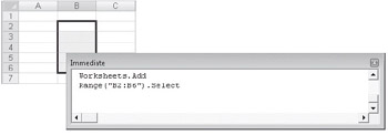
1. In the Visual Basic editor, activate the Immediate window, type Worksheets.Add, and press Enter to create a new, blank worksheet in the active workbook.

2. Type Range("B2:B6").Select and press Enter to select a sample starting range of cells.

   

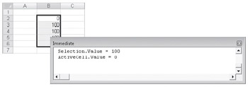
3. Type Selection.Value = 100 and press Enter to fill all the cells of the selection with the number 100.

   Value is a property of the range. When you set the Value property in conjunction with a multicell range, you change all the cells in the range.

   Tip 

   When assigning a contant value to a range, the Formula property is equivalentto the Value property, so Selection.Formula = 100 is the same as Selection.Value = 100. The Formula property is equivalent to whatever you see in the formula bar when the cell is selected. The formula bar can contain constants as well as formulas, and so can the Formula property. When you assign a value to a cell, the Formula property and the Value property have the same effect.

4. Type ActiveCell.Value = 0 and press Enter to change cell B2 to 0.

   Only the active cell changes, not the selected cells. Entering a value in the active cell is equivalent to typing a value and pressing Enter. Entering a value in the selection is equivalent to typing a value and pressing Ctrl+Enter.

   

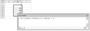
   Suppose you want to enter a value in the cell above the active cell, whatever the active cell might be.

5. Type ActiveCell.Offset(-1).Value = 1 and press Enter to change the value in cell B1 to 1.

   This statement starts with the active cell, uses the Offset property to calculate a new cell one up from that starting cell, and then sets the Value property for the resulting cell.

   

6. Type Selection.FormulaR1C1 = "=R[-1]C*5" and press Enter.

   

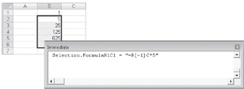
   Now each of the selected cells contains a formula, not a constant. The FormulaR1C1 property expects a formula in R1C1 reference style. The reference R[-1]C always means “one cell above” regardless of which cell gets the formula.

7. Type ?ActiveCell.Value and press Enter.

   This statement displays the value 5 in the Immediate window. The Value property retrieves the result of any formula in a cell. When you retrieve the contents of the cell that contains a formula, the Value property gives you the result of the formula.

8. Type ?ActiveCell.Formula and press Enter.

   This statement displays the formula =B1*5 in the Immediate window. When you retrieve the contents of a cell that contains a formula, the Formula property gives you the formula using A1 reference style. The setting in the Excel Options dialog box is ignored. If you want to retrieve the formula using R1C1 reference style, use the FormulaR1C1 property.

All cells have Formula, FormulaR1C1, and Value properties. The Value property and the Formula property behave the same when you’re writing to the cell. When you read the value of a cell, the Value property gives you the value, and the Formula property gives you the formula using A1 reference style. The FormulaR1C1 property is the same as the Formula property, except that it uses R1C1 reference style for all references, whether assigning a formula to the cell or reading the formula from a cell.

Tip 

The Value property always gives you the unformatted value of the number in a cell. A cell also has a Text property, which returns the formatted value of the cell. The Text property is read-only because it’s a combination of the Value property and the NumberFormat property. A range also has a Value2 property. The difference between Value and Value2 has to do with dealing with very large, very precise numbers-as in banking. The Value property uses a data type (double-precision floating point) that can handle either very large numbers or very precise numbers, but not at the same time. The Value2 property uses a data type (currency) that can handle the large-scale precision needed in financial summaries.

Construct Formulas to Fill a Grid

Sometimes you need a macro to create formulas that contain references. For example, suppose want to create a macro that will enter the appropriate formulas into the Revenue grid. You could just record a macro, but a recorded macro will use specific cell addresses. Suppose that the grid could be anywhere on the worksheet-not just starting in cell A1-and that it could be of any size. Your recorded macro can’t handle that kind of variation.

If you can make a few simple assumptions, you can create a macro that will find a grid, select the current region to find the size of the grid, and then add the correct formula. You can even have the macro automatically find the location of the Discount cell and assign a name to it so that the formula can reference the cell by name. The assumptions you need to make are very useful for most simple macros:

• Always use the consistent words as labels so you can have the macro search for them.

• Always keep the same number of header columns and rows.

• Separate ranges are separated by at least one empty row or one empty column so that the CurrentRegion method can detect the rectangle.

On the Revenue worksheet, the searchable labels are Price and Discount, the grid has two header rows and one header column, and the ranges are separated by column F. With those simple assumptions, you can create a macro that will automatically create the right formula and put it into the correct range.

1. Make a copy of the Revenue worksheet in the Chapter04 workbook, with cell A1 selected.

   Copying the worksheet will give you a chance to test the macro, moving and resizing the revenue grid.

2. In the Visual Basic editor, enter the following macro shell, and press F8 twice to step to the End Sub statement.

   Sub FillFormulas()   Dim myOuter as Range   Dim myInner as Range   Dim myFormula as String End Sub() 

   Declaring variables at the top will make it easier to work with different ranges. The myOuter range will refer to the entire current region of the Revenue grid, including the headings. The myInner range will refer to the empy cells in the middle that need formulas. The myFormula string will contain the formula so that you can construct the formula piece by piece in the macro.

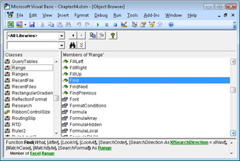
3. In the Object Browser, select Range in the Classes list. Then, in the list of members, select the Find method.

   The description indicates that this property has one required argument-the string you’re searching for-and that it returns a reference to a range.

   

4. In the Immediate Window, type Set myOuter = Cells.Find("Price").CurrentRegion and then press Enter. When you can confirm the correct range by entering myOuter.Select, copy the statement into the macro.

   

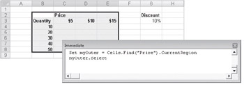
   See Also 

   The Intersect and Offset functions are described in the section titled “Refer to a Relative Range” earlier in this chapter.

   For the myInner range, you need to remove two header rows at the top and the one header column at the left. You can do that by using the combination of Intersect and Offset.

5. In the Immediate window, type Set myInner = Intersect(myOuter,myOuter.Offset(2,1)) and press Enter. When you can confirm the correct range by entering myOuter.Select, copy the statement into the macro.

   

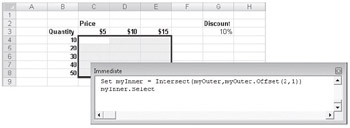
   For the Discount range, you can use the label in the top cell to define the name for the lower cell. This creates a name in the worksheet, rather than a variable in Visual Basic. You assign the name by using the CreateNames method. The CreateNames method has four arguments, Top, Bottom, Left, and Right, respectively. These identify which side of the range contains the labels you should use as names.

   The Discount label is above the discount value, so Top is the only one you need to designate as True. Since Top is the first argument, you can simply omit the others.

6. In the Immediate window, type Cells.Find("Discount").CurrentRegion.CreateNames True and press Enter. When you can confirm the correct range by entering Range("Discount").Select, copy the statement into the macro.

   

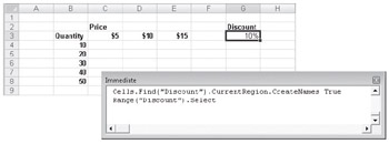
   For the first part of the formula, you need a reference to the first Price cell, which is currently cell C3. If you think of myOuter as if it were a worksheet, you want cell “B2” of that imaginary worksheet, and you want the address in R1C1 notation, with an absolute row number and a relative column number, from the point of view of the first formula cell. The Address method gives you the address of a cell, with arguments to control what it looks like. Visual Basic prompts you for each of the arguments.

7. In the Immediate window, type

   myFormula = myOuter.Range("B2").Address(True,False,xlR1C1,False,myInner) and press Enter. Move the mouse pointer over the word myFormula to confirm that the address is R3C, and then copy the statement into the macro.

   

   Tip 

   When you use the Range method, Visual Basic shows you tips for the methods and properties that follow. When you use the Cells method, Visual Basic does not show tips. Even though Range("B2") and Cells(2,2) are functionally equivalent, using the Range method makes the statement easier to type. If you find the Cells method easier to understand, you can make the change after you have successfully created the statement.

8. In the Immediate window, type myFormula = "=" & myFormula & "*". Move the mouse pointer over the word myFormula to confirm that the value is =R3C*, and then copy the statement into the macro.

9. Enter the following three statements into the macro, optionally testing each one first in the Immediate window.

   myFormula = myFormula & _   myOuter.Range("A3").Address(False, True, xlR1C1, False, myInner) myFormula = myFormula & " * ( 1 - Discount ) " myInner.FormulaR1C1 = myFormula 

   There is nothing fundamentally new in these statements. The first one appends the quantity address, with relative column and absolute row. The second one adds the Discount portion of the formula. The Discount portion doesn’t need to be converted to an address because it’s already a name in the worksheet. The third statement assigns the finished formula to the inner range.

10. Create a new copy of the Revenue worksheet, and test the macro. Then make another copy, change the size and location of the revenue grid, and test the macro again.

    

    Filling ranges of variable sizes with formulas is a powerful technique. You can usethe methods and properties of the Range object to create the formula and to find the correct range to fill.