The Switching Process

All of the descriptions of the switching process contain the same words and phrases. We hear people using terms such as “wire speed” and “low latency,” but these expressions don’t tell us what is going on inside the switch, only how long it takes to happen! If you are anything like me, you want to know what goes on inside. But the inside of a switch is not like the inside of the family auto—taking it to bits doesn’t always let you see the interesting stuff. Let me explain.

When frames arrive at an ingress interface, they must be buffered. Unless the switch is operating in cut-through or fragment-free mode, the frame check sequence needs to be calculated and tested against the arriving FCS. After the frame is confirmed as uncorrupted, it must be passed to a switching “fabric” of some sort, where it can go through the forwarding process to the egress interface.

This forwarding will be expedited by a table lookup process, which must be very quick if the frame is not to be delayed. Finally, there may be contention for the egress interface, and the frame will have to be held in a buffer until the output channel is clear. This complete process will involve a number of discrete steps taken by specific devices.

Note 

I am using the term switching fabric here for two reasons. First, you will hear the term used throughout the industry, often by people who are not quite sure what it means, but who will expect you to know. Second, because it is a broad descriptive term, without a single definition, and because I also intend to use it throughout this chapter. What I mean is the “heart” of the switch, where frames are redirected to an outgoing interface. It might be a crossbar, a bus, or shared memory. Read on and see what I mean.

Switch Architecture and Components

Switches come in a variety of shapes and sizes, as you would expect; after all, as long as the standards are complied with when stated, how you make that happen can be entirely proprietary. And Cisco, which has a range of switches in the portfolio—some designed in-house and others the result of canny purchases—has more than one type of switch.

Modern switches differ from bridges because they support micro-segmentation, and because they do everything very quickly. So they have to be both scalable and efficient, which means that the architecture needs to be designed for the job. You can’t make a world-class switch by purchasing chips from the corner shop and soldering them together.

So modern switches have a number of key components designed for specific purposes, and an architecture that describes how they are connected together.

Non-Blocking Switches

The term non-blocking comes from the telecommunications industry, specifically that section concerned with telephone exchange design. It means that the non-blocking switch must have sufficient capacity in the switching fabric to be able to avoid delaying the frame forwarding. Figure 10.1 shows a non-blocking switch architecture, with eight Gigabit Ethernet interfaces and a 4Gb fabric. This would be the minimum fabric to be truly non-blocking.

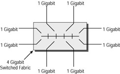
Figure 10.1: Non-blocking switch fabric

Note 

The comparison to telephone exchanges is worth following up, especially as we move toward VoIP. How often do you try to make a telephone call these days and get a tone that says “the exchange is busy”? Not very often, I’ll bet. That is because modern telephone exchanges are non-blocking. But it wasn’t always so. It has taken exchange and network designers some years to get to this advanced stage. And in the data communications industry, we are not there yet!

Now, it doesn’t take too much effort to see that there are really only two ways to create this type of switch. You could use a crossbar, which has a cross-point for every possible interface pair in any given frame-forwarding action (crossbars are described fully in the next section), or you could have some sort of shared memory coupled to a multi-tasking operating system (also in the next section). Everything else will result at some time in a frame being queued because the fabric is busy. This has led to the rise of the term “essentially non-blocking.”

Switches that are essentially non-blocking are so described because the manufacturers deem that the chances of frames being delayed in the fabric, or of any delays being significant, are almost non-existent. This gives the designers of such switches more leeway, and opens the door for fabrics comprising bus architectures.

Tip 

The term “essentially non-blocking” is statistically sound when applied to telephone networks, as it sometimes is. That’s because we can predict with some accuracy the distribution of telephone calls throughout the network across the day. This is less predictable with data, and some forwarding delays will occur. You have to keep an eye on your switch port statistics to ensure that it is not a problem on your network.

Non-blocking switches are sometimes referred to as wire speed switches, in an attempt to explain that, in the absence of any other delays, the switch can forward data at the same rate as which it is received.

Switch Fabrics

There are three main switch fabrics in use today: bus, shared memory, and matrix. Each has its own advantages and disadvantages, and manufacturers select designs based upon the throughput demanded by the switch and the cost required to achieve it.

Bus Switching Fabric

A bus fabric involves a single frame being forwarded at a time. The first issue that this raises is one of contention. Although the frames could be forwarded on a first-come first-served basis, this is unlikely to prove “fair” to all ports, and so most bus fabrics have a contention process involving a second bus just used for contention and access. The most common approach is for an ingress buffer to make a request for access to the forwarding bus when there is a queued frame. The resulting permission from some central logic allows the buffer to forward the frame to the forwarding bus.

Of course, this forwarding bus need not be a simple serial affair, where bits are transmitted one after the other. As the whole frame is already stored in a buffer prior to being forwarded, the bus could be parallel, allowing the frame to be forwarded much more quickly. For example, a 48-bit- wide bus clocked at only 25MHz would result in a possible throughput of 1.2Gbs/second.

Figure 10.2 shows four line cards connected to a shared bus switching fabric.

Figure 10.2: Bus switching fabric

Shared Memory Switching Fabric

Shared memory fabrics pass the arriving frame directly into a large memory block, where all of the checking for corruption is carried out. Corrupted frames are discarded from here.

The header of the frame is checked against the bridging table on the processor, which has direct access to the shared memory. The forwarding decision results in the frame being forwarded to the egress port, and scheduling or prioritization will be managed as the frame leaves the shared memory.

One advantage of shared memory fabrics is that the frame may only have to be queued once as it passes through the switch. Under light loads, very high throughput can be achieved from such architecture. In addition, the line cards don’t need to have the same level of intelligence as with bus architectures, because there is no requirement for a contention mechanism to access the fabric.

Figure 10.3 shows four line cards connected to a shared memory fabric.

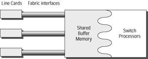
Figure 10.3: Shared memory switching fabric

Crossbar Switching Fabric

Crossbar switching uses a fabric composed of a matrix. In other words, the core of the switch is a series of cross-points, where every input interface has direct access to the matrix, resulting in a truly non-blocking architecture. This design is at the heart of many telephone switches.

What is common, however, is to reduce the size of the matrix by not giving every port its own path to the matrix, but instead giving every line card direct access. Of course, some prioritization and contention management is needed on the line cards, but the system is still extremely fast. Add to this the additional availability created by a second matrix (with line cards attached to each), and you might rightly refer to it as “essentially non-blocking.”

Figure 10.4 shows the basic arrangement for a group of line cards connected to a single crossbar switch.

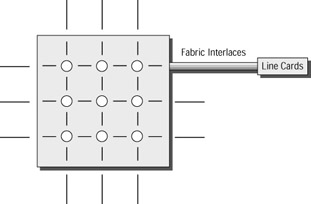
Figure 10.4: Crossbar switching fabric

Bridging Table Operation

Naturally, the bridging table is one of the most important parts of a switch. There is little point in being able to forward data at wire speed if it takes ages to make a decision as to where to forward it. The main mechanisms for table lookup in use today are the Content Addressable Memory (CAM) and the Ternary Content Addressable Memory (TCAM).

Content Addressable Memory (CAM)

CAM is not unique to Cisco, but is almost an industry standard mechanism for how the lookup process for data operates in modern devices. CAM is not the same as a traditional indexing method. These older mechanisms use a pointer to identify the location in memory of specific information (such as an address/port match).

With CAM, a precise relationship exists between the information in the data and its location in the data store. This means that all data with similar characteristics will be found close together in the store. CAM could therefore be defined as any kind of storage device that includes some comparison logic with each bit of data stored.

CAM is sometimes called associative memory.

Ternary Content Addressable Memory (TCAM)

In normal CAM lookups, all of the information is important—in other words, there is nothing you wish to ignore. This is a function of the fact that binary has just the two bits, “ones” and “zeros.” This is restricting, because time must be spent looking for a match for the whole data structure, 48 bits in a MAC address and 32 bits in an IP address.

Ternary mechanisms add a third option to the binary possibilities, that of “don’t care,” commonly shown as the letter X. This means that data can be searched for using a masking technique where we want to match 1s and 0s and ignores Xs.

For example, in a standard CAM, a lookup for the IP address 172.16.0.0 would require a match of 32 bits of 1s and 0s. But if we were trying to find a match on the network 172.16.0.0/16, then we really only need to match the first 16 bits. The result is a much faster lookup because we only have to search for the bits we want to match—extraneous bits would be flagged with a mask of Xs.

TCAMs are useful when there may be bits in a lookup that we can afford to ignore. Good examples are layer 2 and layer 3 forwarding tables and access control lists.

Memory

One of the most important aspects of a switch is the memory. Switches are often presented with interfaces running at different speeds. In fact, the differences are commonly factors of 10 (10/100/1000 Ethernet). Combined with this possible bandwidth mismatch between interfaces, the fact that switches move frames from one interface to another at very high speed means that buffer space can fill up very quickly. The result is that the science of data buffering is quite advanced, and the simple serial shift-register memory of the past is no longer suitable.

The reason for using fixed-size buffers in the first place is not necessarily intuitive. You might think that better use would be made of shared memory by just placing arriving frames/packets into the next free space and making an entry in a table, rather like the way your hard drive manages files. But the problems that arise from this are in fact very similar to the hard drive file storage mechanism. In short, how do we use space that has been released after data has been forwarded from memory?

Obviously, the space made available after a packet has left the memory block is likely to be the wrong size to exactly fit the next occupant. If the next packet is too small, space will be wasted. If it is too large, it won’t fit, and we would need to fragment it. After a while, throughput would slow down and more and more packets would have to be chopped up for storage and reassembled for transmission. On our hard drive, we’d have to defragment our disk regularly. In shared memory, we’d just end up with smaller and smaller memory spaces, with the resulting loss of throughput.

Fixed size buffers allow us to control the way that memory is allocated.

Rings

In order for arriving packets to be placed into the shared memory buffers, it is common to use a buffer control structure called a ring. Shared memory devices usually have two rings, one to control the receive packet buffering and one to control transmit packet buffering.

Rings act effectively as a control plane (if you have a telecommunications background, think out-of-band signaling) that carries information about which frame may go where.

Contiguous Buffers

Contiguous buffers are fixed-size buffers where different units of data (frame, packet, and so on) are placed in separate buffers. This has the advantage of creating easily addressed blocks where data can quickly be both stored and accessed efficiently. In general, contiguous buffers are easy to manage. But there is also a disadvantage in that considerable space can be wasted if, for example, a 64-byte frame has to be placed into a 1500-byte buffer.

On Cisco switches (and routers) that use this method, the contiguous buffers are created in a variety of fixed sizes at startup of the switch. The size of the contiguous buffers is designed to be suitable for a variety of frames/packets of common sizes to be properly stored with the minimum of wasted space.

Note 

The contiguous buffering allocation can be most wasteful on routers, where the need to create buffers to support the MTU of all interfaces may mean that some buffers as large as 18 kilobytes may be reserved (FDDI or high-speed token ring, for example). Under these circumstances, very few frames or packets may demand a buffer this large, but once created, the memory is not available for other purposes. And the maximum memory on switches and routers may be quite limited.

Figure 10.5 shows the disadvantages of the contiguous buffering system. Despite the different- sized buffers that have been created, there is always going to be waste.

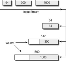
Figure 10.5: Contiguous buffering

Shown next is the output of the show buffers command executed on a WS-C2950-24 switch. You can see the sizes of the system buffers, and the default number that are created at startup by this particular switch.

Terry_2950#show buffers Buffer elements:    500 in free list (500 max allowed)    58 hits, 0 misses, 0 created Public buffer pools: Small buffers, 104 bytes (total 52, permanent 25, peak 52 @ 00:16:09):    52 in free list (20 min, 60 max allowed)    50 hits, 9 misses, 0 trims, 27 created    0 failures (0 no memory) Middle buffers, 600 bytes (total 30, permanent 15, peak 39 @ 00:16:09):    30 in free list (10 min, 30 max allowed)    24 hits, 8 misses, 9 trims, 24 created    0 failures (0 no memory) Big buffers, 1524 bytes (total 5, permanent 5):    5 in free list (5 min, 10 max allowed)    4 hits, 0 misses, 0 trims, 0 created    0 failures (0 no memory) VeryBig buffers, 4520 bytes (total 0, permanent 0):    0 in free list (0 min, 10 max allowed)    0 hits, 0 misses, 0 trims, 0 created    0 failures (0 no memory) Large buffers, 5024 bytes (total 0, permanent 0):    0 in free list (0 min, 5 max allowed)    0 hits, 0 misses, 0 trims, 0 created    0 failures (0 no memory) Huge buffers, 18024 bytes (total 0, permanent 0):    0 in free list (0 min, 2 max allowed)    0 hits, 0 misses, 0 trims, 0 created    0 failures (0 no memory) Interface buffer pools: Calhoun Packet Receive Pool buffers, 1560 bytes (total 512, permanent 512):    480 in free list (0 min, 512 max allowed)    56 hits, 0 misses Terry_2950# 

Warning 

You can change the buffer allocations by using the buffers buffer_size buffer_setting number command, but this is a skilled task with considerable ramifications. If too much memory is allocated to buffers, performance will suffer. If you think you need to alter the default buffer allocations, either liaise with the Cisco TAC or, at the very least, model the impact on a non-production switch.

Particle Buffers

Particle buffers are a new mechanism designed to overcome the limitations of the contiguous buffering system. Instead of allocating a contiguous block, particle-based systems allocate small, discontiguous blocks of memory called particles, which are then linked together to form a logically contiguous packet buffer. These packet buffers are therefore spread across multiple physical particles in different locations.

The advantage of this method is that no buffers of specific sizes need to be allocated in advance; instead, buffers are created as needed, and of the optimum size (within the limits of the particle sizes, which are usually split into pools of 128 and/or 512 bytes).

Figure 10.6 shows how the use of particles may not completely eliminate waste, but sure cuts it down to a minimum!

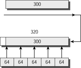
Figure 10.6: Particle buffers

Software

At the heart of the switch is the software. At the moment, a variety of different images appear in the range. This is partly because Cisco is in a transitional stage between the legacy operating systems of the older switches and the completion of the migration toward IOS-based switches. It is also partly because some switches do more than just layer 2 switching. The minute a switch operates at layer 3, it is, in effect, a router as well—which means a router-compliant IOS.

The two main issues that you must understand when considering software are

• On a 2950 switch, is the IOS Standard Image (SI) or Enhanced Image (EI)?

• On a 4000 or 6500 series switch, is the IOS a hybrid of CatOS and IOS, or is it true IOS?

2950 Series Software

Taking the first subject first, Cisco produces the IOS for the 2950 in two versions, Standard Image and Enhanced Image. The images are platform dependent, and when you buy a switch with SI installed, you cannot upgrade to EI.

Standard Image IOS

The SI is installed on the 2950SX-24, 2950-12, and 2950-24. The SI supports basic IOS functionality, and includes functionality to support basic data, video, and voice services at the access layer. In addition to basic layer 2 switching services, the SI supports:

• IGMP snooping

• L2 CoS classification

• 255 multicast groups

• 8000 MAC addresses in up to 64 VLANs

Enhanced Image IOS

The EI is installed on the 2950G-12, 2950G-24, 2950G-48, 2950G-24-DC, 2950T-24, and 2950C-24. The EI supports all features of the SI, plus several additions, including enhanced availability, security, and quality of service (QoS). In addition to the services provided by the SI, the EI supports:

• 8000 MAC addresses in up to 250 VLANs

• 802.1s Multiple Spanning Tree Protocol

• 802.1w Rapid Spanning Tree Protocol

• Gigabit EtherChannel

• Port-based Access Control Lists

• DSCP support for up to 13 values

• Rate limiting on Gigabit Ethernet

  Tip 

  A full breakdown of the components of both the SI and EI images is available at Cisco’s website: www.cisco.com/en/US/products/hw/switches/ps628/prod_ bulletin09186a00800b3089.html.

4000 and 6500 Series Software

The 6500 and 4000 series routers are the ones most exposed to the changing face of Cisco operating systems. Coming from a history of native CatOS, they have moved to a hybrid CatOS/IOS operating system, on the path to becoming fully IOS supported. These changes have brought with them increased functionality and faster throughput.

CatOS/IOS Hybrids

The native operating system on the two platforms has always been CatOS, with the familiar set, show, and clear commands used for almost all control aspects. The introduction of routing and layer 3 switching features on a separate module created the concept of two operating systems on a single switch.

By using an internal telnet connection, or a separate console port on the front of the introduced module, access is gained to the IOS-based routing engine. The Catalyst 4000 4232-L3 module and the Catalyst 6000 Multilayer Switch Feature Card 1 (MSFC 1) and 2 (MSFC 2) fall into this category.

Native IOS

There are some limitations to running two operating systems, not including the most obvious one of having to understand and remember two different sets of commands. The CatOS was written before Cisco acquired the Catalyst company, and represents a different configuration philosophy. It is cumbersome, unfriendly, and very limited when compared with the Cisco IOS, which is mature and flexible.

It makes sense to be able to integrate the complete layer 2 and layer 3 functionality available in the combined switching engines, and this can only be leveraged through the use of an operating system that understands everything. Enter IOS, ready to run in native format on the integrated platform.

Upgrading the IOS is a well-defined process involving a series of steps:

• Confirm that your platform will support the new IOS.

• Confirm that you have the correct IOS from Cisco.

• Establish a TFTP server that your switch can access.

• Ensure that your switch has sufficient flash memory for the new image.

• Copy the new IOS into flash.

• Reload the switch with the new IOS running.

  Tip 

  A reference document on the Cisco website contains detailed instructions for the step-by-step upgrade process on all platforms (including the old 5000 series switches). It can be found at www.cisco.com/en/US/products/hw/switches/ps700/products_tech_note09186a00801347e2.shtml.