Managing Data for Quality

A foremost rule we have always followed while working in the field is to know your data. Many times we have found an organization’s data abused mainly because those in charge of the data did not know how the data was used. In other words, they did not understand their organization’s data. If you are in control of managing your organization’s data, knowing your data is your first task.

How do you learn about your data and at the same time make certain that it adheres to its purpose? We have taken a three-step approach to working with data that has proven to be quite effective. We will show you how this process can work effectively for you and your data to maintain the quality that you need for your business.

Real World Scenario-Clinical Trial Data

For several years I consulted at a major pharmaceutical company working with clinical study data. There are many phases of clinical trials. Phase I trials test an experimental drug or treatment in a small group of people (20–80) for the first time to evaluate its safety, determine a safe dosage range, and identify side effects. Phase II and III trials treat larger groups of people (100–300 and 1,000–3,000), studying the drug or treatment to monitor its effectiveness, side effects, value, and safety. Data is kept in the same database, often in overlapping tables.

The lead programmer for Phase III trials and one of the DBAs for the ClinTrial database ran a script one evening to clean up data on an ongoing study that involved several individual trials. Both individuals had tested the script on a sampling of data from the clinical Phase III trials.

The DBA did not know his data. What he failed to take into account was that Phase I tables were affected and consequently corrupted by the programmer’s script.

Since I was consulting in Phase I studies, I noticed a problem with our data the first thing the next day. However, because of the types of changes made and the need to comply with business requirements, the correction could not be handled by a simple restore process. Consequently, not only were many hours diverted to bringing Phase I data back online, but also studies fell behind schedule while the matter was being corrected.

So, my first rule is take the time to know your data.

-Marilyn Miller-White

Your data as well as the database and objects built upon it are all living and changing entities (see Figure 7.1). Therefore, this process is a continuum; it consists of assessing the data by capturing the business requirements, verifying the data meets quality standards, and validating the data as it’s used and updated.

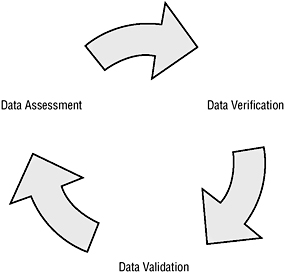
Figure 7.1: The life cycle for data quality

The data in your enterprise-or even your database, for that matter-does not move through the process all at one time or as an entire object. Nor does the process end for a piece of data or an object if it is no longer useful; this entity must be archived and documented. So, not only is the process continuous but the data loop itself is an infinite Mobius band.

Note 

An interesting fact is that Mobius is a well-known company that has long been associated with data management. Most recently, Mobius Management Systems, Inc., has created a technical alliance with Microsoft for enhancing its data management capabilities with Microsoft Office SharePoint Server 2007.

Documenting Your Actions

Before the process begins, we want to make certain you have adhered to the commonsense practice of keeping your work well documented and in one location. For example, you could use sections and forms in a run book for this purpose. It does not matter how your organization, team, or you alone decide to keep records of the process and consequent jobs and outcomes involved. What does matter is that the records are consistently entered and kept up-to-date. It can be the task of one or many; however, it must be a task that is valued. You cannot think of documentation as part of your job description that is “above and beyond”; it needs to be well defined and measured.

Documentation has often been a manual effort for most database administrators. But the database administrator of yesterday is not the DBA of today. Today’s DBA manages all aspects of the database. We’ve even heard some DBAs refer to themselves as internal consultants to developers. At the other end of the spectrum, we’ve heard DBAs complain that they seem to need and understand more code to do their job. As you have been reading the material in this study guide, you’ve probably noticed that there is no longer a fine line between the two positions. To manage your data, you need to be in control of all its characteristics.

Assessing the Data

How can you best get to know and analyze the data? The data you capture needs to go beyond merely being accurate. The data must bring to the public and your customers a reliable and unbiased view of your enterprise. You must develop measures to learn the implicit requirements that are placed on the data. You need to know the data sources and how the data is used. You must communicate with those who interact with the data.

Get to know the players first. They will be able to provide firsthand information about the data. The players you need to interact with include the data producers, the data custodians, and the data consumers:

• Data producers generate and provide the data.

• Data custodians provide and manage computing resources for storing, maintaining, and securing the data.

• Data consumers access and use the data.

Here are the considerations we have found most useful when gathering information and capturing requirements:

• Consult with data management personnel.   To make certain you have a clear understanding of the data flow, the security policies that must be enforced, and the applications that are used by the data, you need to meet with business managers as well as those in charge of the data. They will give you the direction for the quality and regulations that you must consider. It is important to have targeted questions during interviews, which will enable you to start a list of action items to be completed and reviewed by all stakeholders at the end of the requirements process.

• Interact with knowledge workers.   In our experience, interviewing those working directly with the data allows you to really know how the data is used. The users are the real stakeholders; managing the data is their livelihood. They are able to show you what standards are actually in place and give solid opinions on improvements they would like to have available to them from their perspective. Again, we recommend you create a set of targeted questions during your interview process that you can turn into action items at the end of the requirements process.

• Review business and regulatory requirements.   You must consult with the legal department of your organization to obtain the requirements that are imposed upon your data. These requirements can come from a variety of sources. Regulatory acts at many government levels might affect your data; likewise, there might be regulatory acts on the database itself. The legal department also should help you identify all business and security requirements necessary to the business. Make certain that all documents obtained are noted and stored appropriately.

• Evaluate risks.   There are bound to be gray areas where immediate decisions are not readily available. For example, you might have data that is complex and difficult to evaluate, yet you want to include it in your database. You must make certain that you have listed these exceptions and delineated possible plans of actions. It is always better to evaluate the risks up front. Sometimes, by doing so during the review process, you are able to eliminate or at least minimize the risk.

• Follow up with a review meeting with all the stakeholders.   Review your documentation with all stakeholders. You must make certain that you have a clear picture. These people are now part of your team. It is important that you all feel ownership of the document you have put together regarding the data. We have found that ownership is a key factor in the success of many projects. Make certain the review session stays focused and positive. You may want to restate your purpose for all the interviewing and restate your main goal for the project-you want to know your data!

Verifying the Data

Business is built on ensuring data confidence. Each data object has its unique characteristics upon creation and updating. The metadata defines those properties. However, some pieces of data are very complex or abstract, whereas others might be difficult to evaluate. These data entities are most likely included in the risk section of your assessment document. This means you have minimized the risk for those entities and now need to keep an even closer eye on the data as it is processed.

Data Quality Attributes

Data can have various quality attributes. Traditional standards measured such attributes as accuracy, correctness, completeness, and relevance. By today’s data quality standards, those criteria are not sufficient. The Association for Computing Machinery (ACM) has a list of almost 200 terms that serve as criteria, concepts, or goals that describe desirable attributes of data. Table 7.1 represents the criteria we consider most important for you to apply.

Table 7.1: Data Quality Attributes
Open table as spreadsheet

Criteria	Definition
Accessibility	Data is available and able to be retrieved quickly and efficiently.
Completeness	Data is complete if information is not missing and is of sufficient breadth and depth for the recorded analysis.
Concise and unique representation	Data is singularly and compactly represented.
Consistency	Data is aligned with itself and is presented in a singular format.
Free of error	Data is accurate, correct, and reliable.
Objectivity	Data is unbiased, unprejudiced and impartial.
Relevancy	Data is applicable and pertinent for the recorded analysis.
Reputation	Data is highly regarded in terms of source and content.
Security	Data access is restricted appropriately.
Timeliness	Data is kept up-to-date.
Understandability	Data is easily comprehended.

The quality of your data and the information it relays to the consumer is not an exact science. It is bound to your organization. The important concept is that you must be able to measure the criteria on your list. With each criterion you choose, you should have a means of measuring that data quality. Once you’ve established those metrics, you can use them to monitor your data quality.

Verifying the quality of your data and maintaining its integrity is an integral part of the continuum of the data assessment, data verification, and data validation cycle.

Quality Management Tools

SQL Server 2005 has several new tools available to developers in both the database and application venues to ensure their development projects meet the designated quality criteria. Since these tools either have been or will be covered in detail elsewhere in your study, we are including only a synopsis of each here, listed by the business attribute tools they embody:

• Database management tools   SQL Server Management Studio is the Business Intelligence tool used for database management. It contains graphical tools plus an enhanced feature script editor to enable you to access, configure, administer, and manage your server and its databases. It provides developers with a method for creating and saving scripts in a solution and source control environment.

• Database development tools   Business Intelligence Development Studio is used for database development. BIDS is an integrated environment for developing business intelligence structures. You can design cubes, data sources, reports, and Integration Services solutions independent of a particular server. BIDS provides you with a rich development environment and enables you to deploy your final product.

• Data storage tools   The Relational Database Engine is the core service for data storage and processing. The database engine has been completely restructured in SQL Server 2005 to enable processing, security, and access support for highly demanding applications.

• Data-mining solution tools   Analysis Services provides you with the capability to design and create data-mining models using a wide variety of industry-standard data-mining algorithms.

• Data extraction, transformation, and load (ETL) platform   Microsoft SQL Server 2005 Integration Services gives you a platform for building data integration solutions, including ETL packages for data warehousing. SSIS works in the BIDS and SSMS environments.

• Server-based reporting tools   SQL Server 2005 Reporting Services provides a web-enabled reporting environment that enables you to create reports that emanate from a variety of data sources. Reporting Services also services the publishing of reports in a variety of formats and subscription services in a secure environment. Developing and deploying reports are handled in BIDS. The Report Server databases are managed within SSMS. The virtual directory for the Report Manager website is managed in IIS. Configuration for Reporting Services is administered through the Reporting Services Configuration Manager.

• Querying, analyzing, and monitoring tools   The query editor in SSMS provides you with an integrated development environment. Other management tools available in SSMS that have been upgraded or redesigned include Activity Monitor, Job Activity Monitor, Replication Monitor, maintenance plans, security, Database Mail, the Database Engine Tuning Advisor, and SQL Profiler. Other configuration tools for SQL Server 2005 include the SQL Server Configuration Manager and the SQL Server Surface Area Configuration.

Also, new tools that work closely with SQL Server 2005 are available to meet your data quality needs:

• Visual Studio 2005   Visual Studio 2005 is a comprehensive development environment intended for developers to build high-performance, multitier applications. Using Visual Studio 2005, you can build a wide variety of Windows-, web-, mobile-, and Office-based solutions.

• BizTalk Server 2006   BizTalk is a business process management server. It enables you to automate and optimize your business processes through a variety of familiar tools that enable your users to design, develop, deploy, and manage those processes. Included within the installed server are integrated management tools, support for web services, and a business activity monitoring (BAM) portal. You can also use BizTalk server to connect to your legacy systems and existing line-of-business applications.

• Office SharePoint Server 2007   This new server to the Microsoft information management scene is a stable and robust platform upon which you can create web-based applications, collaborate with co-workers, and build a portal for your workflow needs, all while staying compliant with regulations and management policies and maintaining security. SharePoint Server 2007 is built on the .NET Framework 3.0 and the Windows Workflow Foundation (WF). It is able to work with both ASP.NET 1.1 and 2.0 Web Parts. It runs on IIS 6.0 and works with SQL Server 2005 including the SQL 2005 BI features.

All the previously mentioned products work together with the core SQL Server 2005 services to provide a well-managed environment for your data.

Validating the Data

Now that you have data processing and storage in place, you must maintain the validity of the data. Data is defined based on the manner in which it is handled. Data is described by the way it’s created, read, updated, and destroyed. This life cycle is often termed the CRUD (create, read, update, and destroy) cycle. Data objects differ in how they are handled within the cycle. For instance, a customer data object is created differently than a product data object. Likewise, updating a customer object is a much different process than updating an order of several hundred products. The data is capturing reality. You must be careful to make certain the initial data metrics are accurate and precise. Therefore, the verification of the data must be a constant part of every step of the CRUD cycle.

In the following section, we will show you some queries you can use to inspect the data during the various phases of create, read, update, and destroy.

Using Queries to Examine the Data

Usually you run queries to generate a result set for a given requirement or application. When you do this, you are seeking the data set that meets a particular set of conditions. In this section, your objective in building queries to inspect data is to learn about the data. You want to see the data that is useful in your applications.

Join technologies let you compare the data between two tables by matching up rows based upon common data. By being able to understand and apply the various join algorithms, you can analyze your data for extra or missing pieces, for duplicates, or for data that should be further cleaned or merged.

In the following sections, we will discuss each type of join and the data they return for your inspection. You will then practice using each with an exercise using the AdventureWorks sample database.

Let’s first take a look at the general concept of the join, which gets its roots from relational algebra. The join is the horizontal merging of two data sets to produce a new result set. Even if you are joining more than two data sets, the joins are processed two at a time.

Using SQL code, the merging of the data is accomplished through the join, which is specified within the FROM portion of the SELECT statement, along with any aggregate statements or WHERE clauses. The SELECT portion of the statement actually accesses the columns from the joined data set.

Here is the partial syntax for the join statement using D1 and D2 as the two data sets:

 FROM D1 <join_type> JOIN D2 ON <on_filter> WHERE where_filter

The join syntax that is most readily used and that we are using in this book is the ANSI SQL 92 standardization, which specifies all the join processing in the FROM clause of the SELECT statement. This syntax is cleaner and more easily understood than older syntax forms.

Using Inner Joins

The inner join returns only those rows that match between the two data sets based on values in the common column. Figure 7.2 shows a Venn diagram, first introduced by British mathematician John Venn in 1881. The figure shows the set relationship for the inner join using the two tables from the AdventureWorks database that you will be joining in the exercise, the Sales.SalesTerritory table and the Sales.SalesPerson table.

As you see, the inner join returns only the common elements based upon the shared column in the data set. Let’s translate this to SQL.

Figure 7.2: The inner join of two data sets

Exercise 7.1 uses the INNER JOIN. You can execute each step as a separate batch. If you are using SQL Server Management Studio, highlight and run each piece of code between the comments and the GO.

Exercise 7.1: Using an INNER JOIN to Inspect Common Data in the AdventureWorks Sales.SalesTerritory and Sales.SalesPerson Tables

The first section of this exercise adds two new rows of data to the Sales.SalesTerritory table that will be used in all the join exercises:

1. Start the exercise using the AdventureWorks database:

    USE AdventureWorks; GO

2. Insert the following values into the Sales.SalesTerritory table:

    INSERT Sales.SalesTerritory VALUES ('New Jersey', 'US', 'North America',100.00,100.00   ,0,0,newid(),getdate()) INSERT Sales.SalesTerritory VALUES ('Texas', 'US', 'North America',100.00,100.00   ,0,0,newid(),getdate())

3. Execute the INNER JOIN:

    SELECT st.Name AS Territory, sp.SalesPersonID FROM Sales.SalesTerritory st INNER JOIN Sales.SalesPerson sp ON st.TerritoryID = sp.TerritoryID ;

Your output will look like the following:

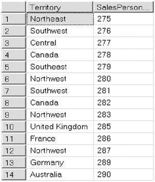
Only territories and their associated salespeople are included in the result set. If a territory has no associated salesperson or if a salesperson has no associated territory, the inner join does not include their data.

Using Left Outer Joins

The outer join extends the inner join by adding the nonmatching data from the left or right data set. Both the left outer join and the right outer join can also be called left join and right join; the term outer can be omitted in the syntax.

Figure 7.3 shows a Venn diagram containing the left outer join of the Sales.SalesTerritory table with the Sales.SalesPerson table.

Figure 7.3: The left outer join of two data sets

All the common data elements are still included in the left outer join but also included are any data elements from the left data set that do not have a match from the right side of the join.

Translating this into SQL, you have what is shown in Exercise 7.2.

Exercise 7.2: Using a LEFT OUTER JOIN to Inspect Data in the AdventureWorks Sales.SalesTerritory and Sales.SalesPerson Tables

Make certain that you have completed the first section of Exercise 7.1, which added two new rows of data to the Sales.SalesTerritory table. We have commented the code for the two inserted rows in this exercise for your review:

1. Start the exercise using the AdventureWorks database:

    USE AdventureWorks; GO

2. Insert values into the Sales.SalesTerritory table completed in the beginning of Exercise 7.1:

    --INSERT Sales.SalesTerritory --VALUES --('New Jersey', 'US', 'North America',100.00,100.00 --  ,0,0,newid(),getdate()) --INSERT Sales.SalesTerritory --VALUES --('Texas', 'US', 'North America',100.00,100.00 --  ,0,0,newid(),getdate())

3. Execute the LEFT OUTER JOIN:

    SELECT st.Name AS Territory, sp.SalesPersonID FROM Sales.SalesTerritory st LEFT OUTER JOIN Sales.SalesPerson sp ON st.TerritoryID = sp.TerritoryID ;

Your output will look like the following:

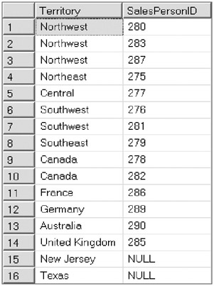
Notice that the left outer join includes the territories of New Jersey and Texas from the Sales.SalesTerritory table that have no associated salesperson in the Sales.SalesPerson table. The rows that have no match contain a null value in the corresponding SalesPerson column. Therefore, if you want to find all the territories, regardless of whether a salesperson is assigned, you would use a left outer join. More appropriately, if you wanted to find the territories that did not have a salesperson assigned, you would use the same left outer join with a WHERE clause. The WHERE clause is a predicate that restricts your output.

Here is the SQL statement:

 -- Execute the LEFT OUTER JOIN with WHERE clause -- to find territories with no salespeople SELECT st.Name AS Territory, sp.SalesPersonID FROM Sales.SalesTerritory st LEFT OUTER JOIN Sales.SalesPerson sp ON st.TerritoryID = sp.TerritoryID WHERE sp.TerritoryID IS NULL;

Your output will look like the following:

Using Right Outer Joins

The right outer join extends the inner join by adding the nonmatching data from the right data set. Figure 7.4 displays a Venn diagram showing the right outer join of the Sales.SalesTerritory table with the Sales.SalesPerson table.

Figure 7.4: The right outer join of two data sets

All the common data elements are still included in the right outer join but also included are any data elements from the right data set that do not have a match from the left side of the join.

Translating this into SQL, you have what’s shown in Exercise 7.3.

Exercise 7.3: Using a RIGHT OUTER JOIN to Inspect Data in the AdventureWorks Sales.SalesTerritory and Sales.SalesPerson Tables

Make certain you have completed the first section of Exercise 7.1, which added two new rows of data to the Sales.SalesTerritory table. We have commented the code for the two inserted rows once again in this exercise for your review.

1. Start the exercise using the AdventureWorks database:

    USE AdventureWorks; GO

2. Insert values into the Sales.SalesTerritory table:

    --Completed in beginning of Exercise 7.1 --INSERT Sales.SalesTerritory --VALUES --('New Jersey', 'US', 'North America',100.00,100.00 --  ,0,0,newid(),getdate()) --INSERT Sales.SalesTerritory --VALUES --('Texas', 'US', 'North America',100.00,100.00 --  ,0,0,newid(),getdate())

3. Execute the RIGHT OUTER JOIN:

    SELECT st.Name AS Territory, sp.SalesPersonID FROM Sales.SalesTerritory st RIGHT OUTER JOIN Sales.SalesPerson sp ON st.TerritoryID = sp.TerritoryID ;

   Your output will look like the following:

   

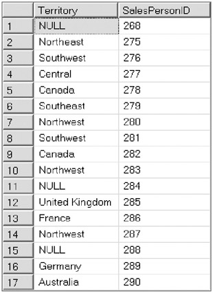
   In this result set, the right outer join includes salespeople from the Sales.SalesPerson table that have no sales territory associated with them from the Sales.SalesTerritory table. The rows that have no match contain a null value in the corresponding Territory column.

4. So, to find all the salespeople regardless of them having a territory, you would use a right outer join. Furthermore, if you needed to find the salespeople who had not been assigned a territory, you could use a WHERE clause to filter the outer join.

5. Here is the SQL statement for the salespeople without a territory:

    -- Execute the RIGHT OUTER JOIN with WHERE clause -- to find the salespeople without a territory SELECT st.Name AS Territory, sp.SalesPersonID FROM Sales.SalesTerritory st RIGHT OUTER JOIN Sales.SalesPerson sp ON st.TerritoryID = sp.TerritoryID WHERE st.TerritoryID IS NULL;

Your output will look like the following:

SalesPersonIDs 268, 284, and 288 do not have a territory assigned to them. A null value is placed in each row of the Territory column for those without a territory.

Using Full Outer Joins

Full outer joins, or full joins, return the results from both data sets regardless of whether a match exists between the two sets.

Figure 7.5 displays a Venn diagram showing the full outer join of the Sales.SalesTerritory table with the Sales.SalesPerson table.

Figure 7.5: The full outer join of two data sets

All the common data elements are still included in the full outer join but also included are all the remaining data elements from both data sets. Furthermore, if there are no common data elements, the full join is just the combination of the two data sets.

You can translate the full outer join into SQL, as shown in Exercise 7.4.

Exercise 7.4: Using a FULL OUTER JOIN to Inspect Data in the AdventureWorks Sales.SalesTerritory and Sales.SalesPerson Tables

Make certain you have completed the first section of Exercise 7.1, which added two new rows of data to the Sales.SalesTerritory table. We have commented the code for the two inserted rows once again in this exercise for your review.

1. Start the exercise using the AdventureWorks database:

    USE AdventureWorks; GO

2. Insert values into the Sales.SalesTerritory table:

    --Completed in beginning of Exercise 7.1 --INSERT Sales.SalesTerritory --VALUES --('New Jersey', 'US', 'North America',100.00,100.00 --  ,0,0,newid(),getdate()) --INSERT Sales.SalesTerritory --VALUES --('Texas', 'US', 'North America',100.00,100.00 --  ,0,0,newid(),getdate())

3. Execute the FULL OUTER JOIN:

    SELECT st.Name AS Territory, sp.SalesPersonID FROM Sales.SalesTerritory st FULL OUTER JOIN Sales.SalesPerson sp ON st.TerritoryID = sp.TerritoryID;

Your output will look like the following:

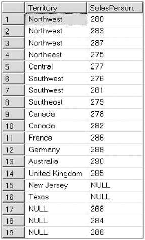
In the result set for the full outer join, the salespeople from the Sales.SalesPerson table and the territories from the Sales.SalesTerritory table are returned, regardless of any common data rows.

4. To go one step further and find the territories and the salespeople not covered, you could once more filter the query using a WHERE clause. However, this time you check whether the TerritoryID in either the SalesTerritory table or the SalesPerson table is null. Here is the SQL statement for the salespeople without a territory and the territories without salespeople:

    -- Execute the FULL OUTER JOIN with WHERE clause -- to find the salespeople without a territory SELECT st.Name AS Territory, sp.SalesPersonID FROM Sales.SalesTerritory st RIGHT OUTER JOIN Sales.SalesPerson sp ON st.TerritoryID = sp.TerritoryID WHERE st.TerritoryID IS NULL Or sp.TerritoryID IS NULL;

Your output will look like the following:

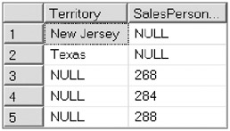
The full outer join as used here with the WHERE filter is useful for returning only the rows in both tables that have no matching data. You can think of this as the negation of the intersection.

Note 

Do you remember DeMorgan’s laws? not(P and Q) = (not P) or (not Q) where (P and Q) is the intersection of sets P and Q.

Using Cross Joins

The cross join is often termed an unrestricted join because it includes all possible combinations of rows from the data sets. The cross join is the Cartesian product of the two sets, that is, the number of row in the first data set multiplied by the number of rows in the second data set. For example, since the modified Sales.SalesTerritory table has 12 rows and the Sales.SalesPerson table has 17 rows, the cross join or Cartesian product of the two tables has their product, or 204 rows.

Note 

The Cartesian product is named after René Descartes, the founder of modern mathematics. His work in analytic geometry as the bridge between algebra and geometry generated this concept.

The SQL syntax for the cross join specifies the CROSS JOIN keywords in the FROM clause. There is no ON condition as in the other join types. Translating this into SQL, you have what is shown in Exercise 7.5.

Exercise 7.5: Using a CROSS JOIN to Inspect Data in the AdventureWorks Sales .SalesTerritory and Sales.SalesPerson Tables

Make certain you have completed the first section of Exercise 7.1, which added two new rows of data to the Sales.SalesTerritory table. We have commented the code for the two inserted rows once again in this exercise for your review.

1. Start the exercise using the AdventureWorks database:

    USE AdventureWorks; GO

2. Insert values into the Sales.SalesTerritory table:

    --Completed in beginning of Exercise 7.1 --INSERT Sales.SalesTerritory --VALUES --('New Jersey', 'US', 'North America',100.00,100.00 --  ,0,0,newid(),getdate()) --INSERT Sales.SalesTerritory --VALUES --('Texas', 'US', 'North America',100.00,100.00 --  ,0,0,newid(),getdate())

3. Execute the CROSS JOIN:

    SELECT st.Name AS Territory, sp.SalesPersonID FROM Sales.SalesTerritory st CROSS JOIN Sales.SalesPerson sp;

   A partial view of your output will look like the following:

   

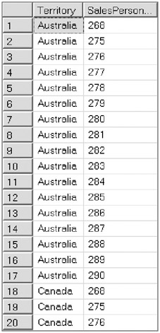
A cross join might not give you an efficient view of your data, but it might come in handy if you need to populate a database with some sample data in a hurry.

Using Sets to Examine Your Data

Many of the join concepts we have presented have their basis in set theory, but you’ve probably guessed that from all our math references! However, some SQL statements are related explicitly to data sets. We’ll discuss those now.

Using Unions

Unions differ from joins in that unions are the additions of the sets whereas joins are the multiplications of the sets. In returning a result set from a join, if we had returned a complete listing of columns from the joined tables, we would have created a very long list in our SELECT statement. The column listing would have been very wide; instead, we decided to choose just two columns, one from each table. With a union, you are adding rows to your data, with no spreading of the columns; union is additive. It vertically appends the one data set to the other. And there may be more-many more-than two sets involved.

The data sets in the union must have the same number of columns, and the lineup of the column data types must be compatible through implicit conversion. The result set uses the column names of the data set named in the first SELECT statement.

The difference between the UNION and UNION ALL operators is that the ALL will include duplicates if they exist. UNION ALL incorporates every row of every data set in the result. If just UNION is specified, duplicates are removed.

Tip 

If you know your data sets contain no duplicates, use UNION ALL instead of UNION. Your query will perform more efficiently since it will not check for duplicates.

Before beginning this set of exercises using the UNION operator, in Exercise 7.6 you’ll create two overlapping tables from the Production.ProductModel table in the AdventureWorks database. The first table will contain those product models with IDs less than 70, and the second table will contain model IDs greater than 50. The original Production.ProductModel table in the AdventureWorks database has 128 entries.

Exercise 7.6: Using UNION and UNION ALL in the AdventureWorks Production .ProductModel Table

First you will create two new tables from this table, Production.ProductModelunder70 and Production.ProductModelover50. Then you will apply UNION and UNION ALL.

1. Start the exercise using the AdventureWorks database:

    USE AdventureWorks; GO

2. Create the Production.Productmodelunder70 table:

    SELECT * INTO adventureworks.production.productmodelunder70 FROM adventureworks.production.productmodel WHERE ProductModelID < 70

3. Create the Production.Productmodelover50 table:

    SELECT * INTO adventureworks.production.productmodelover50 FROM adventureworks.production.productmodel WHERE ProductModelID >50

4. Use the UNION operator on the two tables:

    SELECT ProductModelID, Name from adventureworks.production.productmodelunder70 UNION SELECT ProductModelID, Name from adventureworks.production.productmodelover50

A partial view of your output will look like the following:

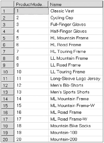
Notice that the UNION operator has removed the duplicates, and that 128 rows, the amount in the original table, are contained in the result set.

5. Use the UNION ALL operator on the two tables:

    SELECT ProductModelID, Name from adventureworks.production.productmodelunder70 UNION ALL SELECT ProductModelID, Name from adventureworks.production.productmodelover50

A partial view of your output will look like the following:

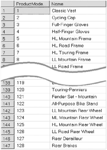
The UNION ALL operator includes the duplicates, so the result set of this query has 147 rows. There are 19 duplicate values.

Using EXCEPT

EXCEPT enables you to identify rows that are in the first data set but not in the second data set. EXCEPT is the only set operator that is asymmetrical. DS1 EXCEPT DS2 is not the same as DS2 EXCEPT DS1. EXCEPT is a tool you can use for comparisons as well as exceptions.

Just as with the UNION set operator, when you use the EXCEPT operator, the number and order of the columns must be the same, and the corresponding data types must be compatible.

In Exercise 7.7 illustrating EXCEPT, you will use the two tables that you created in the previous exercise, Production.ProductModelunder70 and Production.ProductModelover50.

Exercise 7.7: Using EXCEPT in the AdventureWorks Production.ProductModelunder70 and Production.ProductModelover50 Tables

We have included the code, commented out, for creating these tables if you have not created them previously. Then, in the first query, you will apply EXCEPT using Production .ProductModelunder70 as the first data set and Production.ProductModelover50 as the second. In the second query, you will switch the order of the two data sets in the EXCEPT query.

1. Start the exercise using the AdventureWorks database:

    USE AdventureWorks; GO

2. Create the Production.Productmodelunder70 table:

    --SELECT * INTO adventureworks.production.productmodelunder70 --FROM adventureworks.production.productmodel --WHERE ProductModelID < 70

3. Create the Production.Productmodelover50 table:

    --SELECT * INTO adventureworks.production.productmodelover50 --FROM adventureworks.production.productmodel --WHERE ProductModelID >50

4. Use the EXCEPT operator on the two tables, using the production.productmodelunder70 table as the first data set:

    SELECT ProductModelID, Name from adventureworks.production.productmodelunder70 EXCEPT SELECT ProductModelID, Name from adventureworks.production.productmodelover50

A partial view of your output will look like the following:

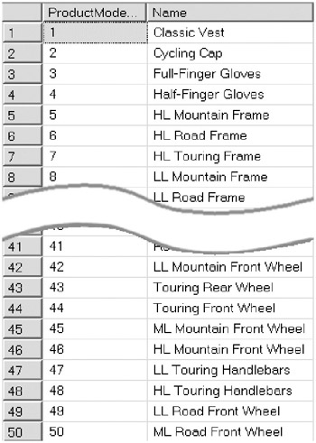
Notice that the result set contains 50 rows with ProductModelIDs ranging from 1 through 50. These ProductModelIDs represent the rows that are in the first data set that are not in the second data set, Production.ProductModelover50.

See what happens when you switch the two data sets around in the EXCEPT statement:

5. Use the EXCEPT operator on the two tables using the production.productmodelover50 table as the first data set:

    SELECT ProductModelID, Name from adventureworks.production.productmodelover50 EXCEPT SELECT ProductModelID, Name from adventureworks.production.productmodelunder70

A partial view of your output will look like the following:

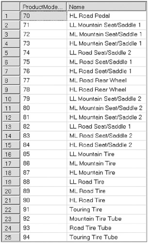
This result set contains 59 rows with ProductModelIDs ranging from 70 through 128. These ProductModelIDs represent the rows that are in the first data set that are not in the second data set, Production.ProductModelunder70.

So when using this statement, you need to make certain you set up the query correctly, especially if the EXCEPT statement is just part of a larger inspection of your data. Remember, EXCEPT is asymmetrical.

Using INTERSECT

INTERSECT returns rows that are common to both data sets. Just as with the other set operations, when you use the INTERSECT operator, the number and order of the columns must be the same, and the corresponding data types must be compatible.

In Exercise 7.8 illustrating INTERSECT, you will use the two tables that you created previously, Production.ProductModelunder70 and Production.ProductModelover50.

Exercise 7.8: Using INTERSECT in the AdventureWorks Production.ProductModelunder70 and Production.ProductModelover50 Tables

In this exercise, we have included the code, commented out, for creating these tables if you have not yet created them. Then you will apply INTERSECT using the Production.ProductModelunder70 and Production.ProductModelover50 tables.

1. Start the exercise using the AdventureWorks database:

    USE AdventureWorks; GO

2. Create the Production.Productmodelunder70 table:

    --SELECT * INTO adventureworks.production.productmodelunder70 --FROM adventureworks.production.productmodel --WHERE ProductModelID < 70

3. Create the Production.Productmodelover50 table:

    --SELECT * INTO adventureworks.production.productmodelover50 --FROM adventureworks.production.productmodel --WHERE ProductModelID >50

4. Use the INTERSECT operator on the two tables:

    SELECT ProductModelID, Name from adventureworks.production.productmodelunder70 INTERSECT SELECT ProductModelID, Name from adventureworks.production.productmodelover50

A partial view of your output will look like the following:

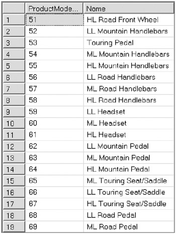
This result set contains 19 rows with ProductModelIDs ranging from 51 through 69. These ProductModelIDs represent the rows that are common to both data sets.

Note 

The EXCEPT and INTERSECT set operators are new to SQL Server 2005. As you have seen, they are both extensions of the UNION operator and as such required a lot more code in previous versions than what you now use to get the same results. Make certain you understand and know how to use these two new keywords.

Using CHECKSUM

In general, CHECKSUM is a redundancy check used to protect data integrity. The checksum itself is an algorithm that adds up the basic components of the data involved, usually the bits, and stores the result in a value. At a later time, an operation desiring to authenticate the integrity of the data can perform the same checksum algorithm and compare the results. If the checksums match, all is in good order. If the checksums do not match, there is a problem with the integrity of the data.

SQL Server 2005 has added CHECKSUM as a protection component of the page verify recovery process. CHECKSUM is now available as an option for discovering and reporting incomplete I/O transactions caused by disk I/O errors. Earlier versions of SQL Server had only the options of TornPageDetection or None to aid in this process. The TornPageDetection option uses a lesser amount of resources than CHECKSUM but does not afford its data protection. Originally introduced with SQL Server 2000, TornPageDetection’s primary focus is detecting page corruptions due to power failures. It notes when only partial sectors are written to disk and detects the incomplete state of the page as it is read from disk.

When you use CHECKSUM, SQL Server creates a checksum for the page contents as they are written to disk. The checksum value is stored in the database page header. When the page is read from disk, its checksum is calculated using the same algorithm and compared with the one stored in the header. If the values do not match, SQL Server assumes that the page has been corrupted, and an error is written to the Windows Event Log.

You set the CHECKSUM database property either by using the Options sheet of the Database Properties page for your database, as shown in Figure 7.6, or by using the ALTER DATABASE Transact-SQL statement.

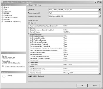
Figure 7.6: Setting the CHECKSUM page verify option

Cleaning the Data

You use data cleansing to ensure your master data has a high degree of consistency and integrity. When you have multiple or disparate data sources, cleansing the data becomes a consuming process. You may have many issues to confront prior to accepting or even beginning the cleansing process. Suppose, for example, that there is no unique identifier across all your data sources. What can you do? Where do you turn? On the other hand, perhaps you have a unique identifier but your data definitions just do not fit with one another. For example, one source may call a financial institution a bank while another uses financial and another uses fin_inst. They might even have names local to the individual business for identical product lines. So, once again, this boils down to knowing your data! But also, you need major assistance with some data-cleansing solutions.

In Chapter 6 you saw how you can use SSIS for solutions just like this. SSIS contains two transformations employing fuzzy logic that you can use:

• Using fuzzy lookups in SSIS   If you already have a well-established set of master data and are trying to match another source of data against this standardized set, you should use a fuzzy lookup transformation. During the performance of the fuzzy lookup, SSIS creates index values for the incoming data matches depicting the amount of relevance to a proposed match, with a value of 1 being a complete match. You can then choose a confidence level at which you will automatically accept data into your existing environment.

• Using fuzzy groupings in SSIS   If you do not have an established set of master data but are merely combining a variety of data sources for a “best fit,” you should use a fuzzy grouping transformation. The algorithms in fuzzy grouping analyze the source data and derive a reference record set. From that point, all records in the data set are evaluated against this newly defined reference set for potential matches.

Using SSIS Data-Cleaning Tools

Other data transformations, such as the conditional split to assist in categorizing the output data based on your business logic, are used quite often in data-cleansing packages. Another is the derived column; this transformation is often applied to a master data set to create a new column definition.

Microsoft offers a data-cleaning sample that uses both the fuzzy lookup and fuzzy grouping transformations as part of the SQL Server samples. You can find the data-cleaning package sample information at http://msdn2.microsoft.com/en-us/library/ms160742.aspx.