Calculating the Number of Paths through a System

The tester needs a systematic way of counting paths by calculation-before investing all the time required to map them-in order to predict how much testing needs to be done. A path is defined as a track or way worn by footsteps, and also a line of movement or course taken. In all following discussions, path can refer to any end-to-end traversal through a system. For example, path can refer to the steps a user takes to execute a program function, a line of movement through program code, or the course taken by a message being routed across a network.

In the series of required decisions example, each side branch returns to the main path rather than going to the exit. This means that the possible branching paths can be combined in 2 × 2 × 2 × 2 = 2⁴ = 16 ways, according to the fundamental principles of counting. This is an example of a 2ⁿ problem. As we saw, this set of paths is exhaustive, but it contains many redundant paths.

In a test effort, it is typical to maximize efficiency by avoiding unproductive repetition. Unless the way the branches are combined becomes important, there is little to be gained from exercising all 16 of these paths. How do we pick the minimum number of paths that should be exercised in order to ensure adequate test coverage? To optimize testing, the test cases should closely resemble actual usage and should include the minimum set of paths that ensure that each path segment is covered at least one time, while avoiding unnecessary redundancy.

It is not possible today to reliably calculate the total number of paths through a system by an automated process. Most systems contain some combination of 2ⁿ logic structures and simple branching constructs. Calculating the total number of possibilities requires lengthy analysis. However, when a system is modeled according to a few simple rules, it is possible to quickly calculate the number of linearly independent paths through it. This method is far preferable to trying to determine the total number of paths by manual inspection. This count of the linearly independent paths gives a good estimate of the minimum number of paths that are required to traverse each path in the system, at least one time.

The Total Is Equal to the Sum of the Parts

The total independent paths (IPs) in any system is the sum of the IPs through its elements and subsystems. For the purpose of counting tests, we introduce TIP, which is the total independent paths of the subsystem elements under consideration-that is, the total number of linearly independent paths being considered. TIP usually represents a subset of the total number of linearly independent paths that exist in a complex system.

TIP = Total enumerated paths for the system

e = element

IP = Independent paths in each element

What Is a Logic Flow Map?

A logic flow map is a graphic depiction of the logic paths though a system, or some function that is modeled as a system. Logic flow maps model real systems as logic circuits. A logic circuit can be validated much the same way an electrical circuit is validated. Logic flow diagrams expose logical faults quickly. The diagrams are easily updated by anyone, and they are an excellent communications tool.

System maps can be drawn in many different ways. The main advantage of modeling systems as logic flow diagrams is so that the number of linearly independent paths through the system can be calculated and so that logic flaws can be detected. Other graphing techniques may provide better system models but lack these fundamental abilities. For a comprehensive discussion of modeling systems as graphs and an excellent introduction to the principals of statistical testing, see Black-Box Testing by Boris Beizer (John Wiley & Sons, 1995).

The Elements of Logic Flow Mapping

	Edges	Lines that connect nodes in the map.
	Decisions	A branching node with one (or more) edges entering and two edges leaving. Decisions can contain processes. In this text, for the purposes of clarity, decisions will be modeled with only one edge entering.
	Processes	A collector node with multiple edges entering and one edge leaving. A process node can represent one program statement or an entire software system.
	Regions	A region is any area that is completely surrounded by edges and processes. In actual practice, regions are the hardest elements to find. If a model of the system can be drawn without any edges crossing, the regions will be obvious, as they are here. In event-driven systems, the model must be kept very simple or there will inevitably be crossed edges, and then finding the number of regions becomes very difficult.

Notes on nodes: 

• All processes and decisions are nodes.

• Decisions can contain processes.

The Rules for Logic Flow Mapping

A logic flow map conforms to the conventions of a system flow graph with the following stipulation:

1. The representation of a system (or subsystem) can have only one entry point and one exit point; that is, it must be modeled as a structured system.

2. The system entry and exit points do not count as edges.

   This is required to satisfy the graphing theory stipulation that the graph must be strongly connected. For our purposes, this means that there is a connection between the exit and entrance of the logic flow diagram. This is the reason for the dotted line connecting the maze exits back to their entrances, in the examples. After all, if there is no way to get back to the entrance of the maze, you can't trace any more paths no matter how many there may be.

The logic flow diagram is a circuit. Like a water pipe system, there shouldn't be any leaks. Kirchoff's electrical current law states: "The algebraic sum of the currents entering any node is zero." This means that all the logic entering the system must also leave the system. We are constraining ourselves to structured systems, meaning there is only one way in and one way out. This is a lot like testing each faucet in a house, one at a time. All the water coming in must go out of that one open faucet.

One of the strengths of this method is that it offers the ability to take any unstructured system and conceptually represent it as a structured system. So no matter how many faucets there are, only one can be turned on at any time. This technique of only allowing one faucet to be turned on at a time can be used to write test specifications for unstructured code and parallel processes. It can also be used to reengineer an unstructured system so that it can be implemented as a structured system.

The tester usually does not know exactly what the logic in the system is doing. Normally, testers should not know these details because such knowledge would introduce serious bias into the testing. Bias is the error we introduce simply by having knowledge, and therefore expectations, about the system. What the testers need to know is how the logic is supposed to work, that is, what the requirements are. If these details are not written down, they can be reconstructed from interviews with the developers and designers and then written down. They must be documented, by the testers if necessary. Such documentation is required to perform verification and defend the tester's position.

A tester who documents what the system is actually doing and then makes a judgment on whether that is "right or not" is not verifying the system. This tester is validating, and validation requires a subjective judgment call. Such judgment calls are always vulnerable to attack. As much as possible, the tester should be verifying the system.

The Equations Used to Calculate Paths

There are three equations from graphing theory that we will use to calculate the number of linearly independent paths through any structured system. These three equations and the theory of linear independence were the work of a Dutch scholar named C. Berge who introduced them in his work Graphs and Hypergraphs (published in Amsterdam, The Netherlands: North-Holland, 1973.) Specifically, Berge's graph theory defines the cyclomatic number v(G) of a strongly connected graph G with N nodes, E edges, and one connected component. This cyclomatic number is the number of linearly independent paths through the system.

We have three definitions of the cyclomatic number. This gives us the following three equations. The proofs are not presented here.

• v(G) = IP = Edges - Nodes + 2 (IP = E - N + 2)

• v(G) = IP = Regions + 1 (IP = R + 1)

• v(G) = IP = Decisions + 1 (IP = D + 1)

Even though the case statement and the series of required decisions don't have the same number of total paths, they do have the same number of linearly independent paths.

The number of linearly independent paths though a system is usually the minimum number of end-to-end paths required to touch every path segment at least once. In some cases, it is possible to combine several path segments that haven't been taken previously in a single traversal. This can have the result that the minimum number of paths required to cover the system is less than the number of IPs. In general, the number of linearly independent paths, IPs, is the minimum acceptable number of paths for 100 percent coverage of paths in the system. This is the answer to the question, "How many ways can you get through the system without retracing our path?" The total paths in a system are combinations of the linearly independent paths through the system. If a looping structure is traversed one time, it has been counted. Let's look at an example.

Refer to the looping structure shown in Figure 11.10. All three equations must be equal to the same number for the logic circuit to be valid. If the system is not a valid logic circuit, it can't work. When inspections are conducted with this in mind, logic problems can be identified quickly. Testers who develop the logic flow diagrams for the system as an aid in test design find all sorts of fuzzy logic errors before they ever begin to test the system.

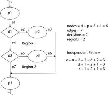
Figure 11.10: Looping structure.

When it is not possible to represent a system without edges that cross, the count of the regions becomes problematic and is often neglected. If the number of regions in a model cannot be established reliably, the logic flow cannot be verified using these equations, but the number of linearly independent paths can still be calculated using the other two equations.

Most of the commercially available static code analyzers use only the number of decisions in a system to determine the number of linearly independent paths, but for the purposes of logic flow analysis, all three equations are necessary. Any one by itself may identify the number of linearly independent paths through the system, but is not sufficient to test whether the logic flow of the system is valid.

Twenty years ago, several works were published that used definitions and theorems from graphing theory to calculate the number of paths through a system. Building on the work of Berge, Tom McCabe and Charles Butler applied cyclomatic complexity to analyze the design of software and eventually to analyze raw code. (See "Design Complexity Measurement and Testing" in Communications of the ACM, December 1989, Volume 32, Number 12.) This technique eventually led to a set of metrics called the McCabe complexity metrics. The complexity metrics are used to count various types of paths through a system. In general, systems with large numbers of paths are considered to be bad under this method. It has been argued that the number of paths through a system should be limited to control complexity. A typical program module is limited to 10 or fewer linearly independent paths.

There are two good reasons for this argument. The first is that human beings don't handle increasing complexity very well. We are fairly efficient when solving logic problems with one to five logic paths, but beyond that, our performance starts to drop sharply. The time required to devise a solution for a problem rises geometrically with the number of paths. For instance, it takes under five minutes for typical students to solve a logic problem with fewer than five paths. It takes several hours to solve a logic problem with 10 paths, and it can take several days to solve a logic problem with more than 10 paths. The more complex the problem, the greater the probability that a human being will make an error or fail to find a solution.

The second reason is that 20 years ago software systems were largely monolithic and unstructured. Even 10 years ago, most programming was done in languages like Assembler, Cobol, and Fortran. Coding practices of that time were only beginning to place importance on structure. The logic flow diagrams of such systems are typically a snarl of looping paths with the frayed ends of multiple entries and exits sticking out everywhere. Such diagrams strongly resemble a plate of spaghetti-hence the term spaghetti code, and the justifiable emphasis on limiting complexity. The cost of maintaining these systems proved to be unbearable for most applications, and so, over time, they have been replaced by modular structured systems.

Today's software development tools, most notably code generators, and fourth-generation languages (4GLs) produce complex program modules. The program building blocks are recombined into new systems constantly, and the result is ever more complex but stable building blocks. The structural engineering analogy to this is an average 100-by-100-foot, one-story warehouse. One hundred years ago, we would have built it using about 15,000 3-by-9-by-3-inch individually mortared bricks in a double course wall. It would have taken seven masons about two weeks to put up the walls. Today we might build it with about forty 10-foot-by-10-foot-by-6-inch pre-stressed concrete slabs. It would take a crane operator, a carpenter, and a welder one to two days to set the walls. A lot more engineering goes into today's pre-stressed slab, but the design can be reused in many buildings. Physically, the pre-stressed slab is less complex than the brick wall, having only one component, but it is a far more complex design requiring a great deal more analysis and calculation.

Once a logic problem is solved and the logic verified, the module becomes a building block in larger systems. When a system is built using prefabricated and pretested modules, the complexity of the entire system may be very large. This does not mean that the system is unstable or hard to maintain.

It is simplistic to see limited complexity as a silver bullet. Saying that a program unit having a complexity over 10 is too complex is akin to saying, "A person who weighs over 150 pounds is overweight." We must take other factors into consideration before we make such a statement. The important factor in complex systems is how the paths are structured, not how many there are. If we took this approach seriously, we would not have buildings taller than about five stories, or roller-coasters that do vertical loops and corkscrews, or microprocessors, or telephone systems, or automobiles, and so on. If the building blocks are sound, large complexity is not a bad thing.

Note 

Complexity is not a bad thing. It just requires structure and management.