31 6.
|  | ||||||
5.1 Costs Associated with Constructed Facilities
The costs of a constructed facility to the owner include both the initial capital cost and the subsequent operation and maintenance costs. Each of these major cost categories consists of a number of cost components .The capital cost for a construction project includes the expenses related to the inital establishment of the facility:
- Land acquisition, including assembly, holding and improvement
- Planning and feasibility studies
- Architectural and engineering design
- Construction, including materials, equipment and labor
- Field supervision of construction
- Construction financing
- Insurance and taxes during construction
- Owner's general office overhead
- Equipment and furnishings not included in construction
- Inspection and testing
- Land rent, if applicable
- Operating staff
- Labor and material for maintenance and repairs
- Periodic renovations
- Insurance and taxes
- Financing costs
- Utilities
- Owner's other expenses
It is important for design professionals and construction managers to realize that while the construction cost may be the single largest component of the capital cost, other cost components are not insignificant. For example, land acquisition costs are a major expenditure for building construction in high-density urban areas, and construction financing costs can reach the same order of magnitude as the construction cost in large projects such as the construction of nuclear power plants.
From the owner's perspective, it is equally important to estimate the corresponding operation and maintenance cost of each alternative for a proposed facility in order to analyze the life cycle costs. The large expenditures needed for facility maintenance, especially for publicly owned infrastructure, are reminders of the neglect in the past to consider fully the implications of operation and maintenance cost in the design stage.
In most construction budgets , there is an allowance for contingencies or unexpected costs occuring during construction. This contingency amount may be included within each cost item or be included in a single category of construction contingency. The amount of contingency is based on historical experience and the expected difficulty of a particular construction project. For example, one construction firm makes estimates of the expected cost in five different areas:
- Design development changes,
- Schedule adjustments,
- General administration changes (such as wage rates),
- Differing site conditions for those expected, and
- Third party requirements imposed during construction, such as new permits .
In this chapter, we shall focus on the estimation of construction cost, with only occasional reference to other cost components. In Chapter 6, we shall deal with the economic evaluation of a constructed facility on the basis of both the capital cost and the operation and maintenance cost in the life cycle of the facility. It is at this stage that tradeoffs between operating and capital costs can be analyzed .
Example 5-1: Energy project resource demands [1]
The resources demands for three types of major energy projects investigated during the energy crisis in the 1970's are shown in Table 5-1. These projects are: (1) an oil shale project with a capacity of 50,000 barrels of oil product per day; (2) a coal gasification project that makes gas with a heating value of 320 billions of British thermal units per day, or equivalent to about 50,000 barrels of oil product per day; and (3) a tar sand project with a capacity of 150,000 barrels of oil product per day.For each project, the cost in billions of dollars, the engineering manpower requirement for basic design in thousands of hours, the engineering manpower requirement for detailed engineering in millions of hours, the skilled labor requirement for construction in millions of hours and the material requirement in billions of dollars are shown in Table 5-1. To build several projects of such an order of magnitude concurrently could drive up the costs and strain the availability of all resources required to complete the projects. Consequently, cost estimation often represents an exercise in professional judgment instead of merely compiling a bill of quantities and collecting cost data to reach a total estimate mechanically.
| | |||
| Oil shale (50,000 barrels/day) | Coal gasification (320 billions BTU/day) | Tar Sands (150,000 barrels/day) | |
| | |||
| Cost ($ billion) | 2.5 | 4 | 8 to 10 |
| Basic design (Thousands of hours) | 80 | 200 | 100 |
| Detailed engineering (Millions of hours) | 3 to 4 | 4 to 5 | 6 to 8 |
| Construction (Millions of hours) | 20 | 30 | 40 |
| Materials ($ billion) | 1 | 2 | 2.5 |
| | |||
| Source: Exxon Research and Engineering Company, Florham Park, NJ | |||
Back to top
5.2 Approaches to Cost Estimation
Cost estimating is one of the most important steps in project management. A cost estimate establishes the base line of the project cost at different stages of development of the project. A cost estimate at a given stage of project development represents a prediction provided by the cost engineer or estimator on the basis of available data. According to the American Association of Cost Engineers , cost engineering is defined as that area of engineering practice where engineering judgment and experience are utilized in the application of scientific principles and techniques to the problem of cost estimation, cost control and profitability.Virtually all cost estimation is performed according to one or some combination of the following basic approaches:
Production function. In microeconomics, the relationship between the output of a process and the necessary resources is referred to as the production function. In construction, the production function may be expressed by the relationship between the volume of construction and a factor of production such as labor or capital. A production function relates the amount or volume of output to the various inputs of labor, material and equipment. For example, the amount of output Q may be derived as a function of various input factors x 1 , x 2 , ..., x n by means of mathematical and/or statistical methods. Thus, for a specified level of output, we may attempt to find a set of values for the input factors so as to minimize the production cost. The relationship between the size of a building project (expressed in square feet) to the input labor (expressed in labor hours per square foot ) is an example of a production function for construction. Several such production functions are shown in Figure 3-3 of Chapter 3.
Empirical cost inference. Empirical estimation of cost functions requires statistical techniques which relate the cost of constructing or operating a facility to a few important characteristics or attributes of the system. The role of statistical inference is to estimate the best parameter values or constants in an assumed cost function. Usually, this is accomplished by means of regression analysis techniques.
Unit costs for bill of quantities. A unit cost is assigned to each of the facility components or tasks as represented by the bill of quantities. The total cost is the summation of the products of the quantities multiplied by the corresponding unit costs. The unit cost method is straightforward in principle but quite laborious in application. The initial step is to break down or disaggregate a process into a number of tasks. Collectively, these tasks must be completed for the construction of a facility. Once these tasks are defined and quantities representing these tasks are assessed, a unit cost is assigned to each and then the total cost is determined by summing the costs incurred in each task. The level of detail in decomposing into tasks will vary considerably from one estimate to another.
Allocation of joint costs. Allocations of cost from existing accounts may be used to develop a cost function of an operation. The basic idea in this method is that each expenditure item can be assigned to particular characteristics of the operation. Ideally, the allocation of joint costs should be causally related to the category of basic costs in an allocation process. In many instances, however, a causal relationship between the allocation factor and the cost item cannot be identified or may not exist. For example, in construction projects, the accounts for basic costs may be classified according to (1) labor, (2) material, (3) construction equipment, (4) construction supervision, and (5) general office overhead. These basic costs may then be allocated proportionally to various tasks which are subdivisions of a project.
Back to top
5.3 Types of Construction Cost Estimates
Construction cost constitutes only a fraction, though a substantial fraction, of the total project cost. However, it is the part of the cost under the control of the construction project manager. The required levels of accuracy of construction cost estimates vary at different stages of project development, ranging from ball park figures in the early stage to fairly reliable figures for budget control prior to construction. Since design decisions made at the beginning stage of a project life cycle are more tentative than those made at a later stage, the cost estimates made at the earlier stage are expected to be less accurate. Generally, the accuracy of a cost estimate will reflect the information available at the time of estimation.Construction cost estimates may be viewed from different perspectives because of different institutional requirements. In spite of the many types of cost estimates used at different stages of a project, cost estimates can best be classified into three major categories according to their functions. A construction cost estimate serves one of the three basic functions: design, bid and control. For establishing the financing of a project, either a design estimate or a bid estimate is used.
- Design Estimates. For the owner or its designated design professionals, the types of cost estimates encountered run parallel with the planning and design as follows :
- Screening estimates (or order of magnitude estimates)
- Preliminary estimates (or conceptual estimates)
- Detailed estimates (or definitive estimates)
- Engineer's estimates based on plans and specifications
- Bid Estimates. For the contractor, a bid estimate submitted to the owner either for competitive bidding or negotiation consists of direct construction cost including field supervision, plus a markup to cover general overhead and profits. The direct cost of construction for bid estimates is usually derived from a combination of the following approaches.
- Subcontractor quotations
- Quantity takeoffs
- Construction procedures.
- 3. Control Estimates. For monitoring the project during construction, a control estimate is derived from available information to establish:
- Budget estimate for financing
- Budgeted cost after contracting but prior to construction
- Estimated cost to completion during the progress of construction.
Design Estimates
In the planning and design stages of a project, various design estimates reflect the progress of the design. At the very early stage, the screening estimate or order of magnitude estimate is usually made before the facility is designed, and must therefore rely on the cost data of similar facilities built in the past. A preliminary estimate or conceptual estimate is based on the conceptual design of the facility at the state when the basic technologies for the design are known. The detailed estimate or definitive estimate is made when the scope of work is clearly defined and the detailed design is in progress so that the essential features of the facility are identifiable. The engineer's estimate is based on the completed plans and specifications when they are ready for the owner to solicit bids from construction contractors. In preparing these estimates, the design professional will include expected amounts for contractors' overhead and profits.The costs associated with a facility may be decomposed into a hierarchy of levels that are appropriate for the purpose of cost estimation. The level of detail in decomposing the facility into tasks depends on the type of cost estimate to be prepared. For conceptual estimates, for example, the level of detail in defining tasks is quite coarse; for detailed estimates, the level of detail can be quite fine.
As an example, consider the cost estimates for a proposed bridge across a river . A screening estimate is made for each of the potential alternatives, such as a tied arch bridge or a cantilever truss bridge. As the bridge type is selected, e.g. the technology is chosen to be a tied arch bridge instead of some new bridge form, a preliminary estimate is made on the basis of the layout of the selected bridge form on the basis of the preliminary or conceptual design. When the detailed design has progressed to a point when the essential details are known, a detailed estimate is made on the basis of the well defined scope of the project. When the detailed plans and specifications are completed, an engineer's estimate can be made on the basis of items and quantities of work.
Bid Estimates
The contractor's bid estimates often reflect the desire of the contractor to secure the job as well as the estimating tools at its disposal. Some contractors have well established cost estimating procedures while others do not. Since only the lowest bidder will be the winner of the contract in most bidding contests, any effort devoted to cost estimating is a loss to the contractor who is not a successful bidder. Consequently, the contractor may put in the least amount of possible effort for making a cost estimate if it believes that its chance of success is not high.If a general contractor intends to use subcontractors in the construction of a facility, it may solicit price quotations for various tasks to be subcontracted to specialty subcontractors . Thus, the general subcontractor will shift the burden of cost estimating to subcontractors. If all or part of the construction is to be undertaken by the general contractor, a bid estimate may be prepared on the basis of the quantity takeoffs from the plans provided by the owner or on the basis of the construction procedures devised by the contractor for implementing the project. For example, the cost of a footing of a certain type and size may be found in commercial publications on cost data which can be used to facilitate cost estimates from quantity takeoffs. However, the contractor may want to assess the actual cost of construction by considering the actual construction procedures to be used and the associated costs if the project is deemed to be different from typical designs. Hence, items such as labor, material and equipment needed to perform various tasks may be used as parameters for the cost estimates.
Control Estimates
Both the owner and the contractor must adopt some base line for cost control during the construction. For the owner, a budget estimate must be adopted early enough for planning long term financing of the facility. Consequently, the detailed estimate is often used as the budget estimate since it is sufficient definitive to reflect the project scope and is available long before the engineer's estimate. As the work progresses, the budgeted cost must be revised periodically to reflect the estimated cost to completion. A revised estimated cost is necessary either because of change orders initiated by the owner or due to unexpected cost overruns or savings.For the contractor, the bid estimate is usually regarded as the budget estimate, which will be used for control purposes as well as for planning construction financing. The budgeted cost should also be updated periodically to reflect the estimated cost to completion as well as to insure adequate cash flows for the completion of the project.
Example 5-2: Screening estimate of a grouting seal beneath a landfill [2]
One of the methods of isolating a landfill from groundwater is to create a bowl-shaped bottom seal beneath the site as shown in Figure 5-0. The seal is constructed by pumping or pressure-injecting grout under the existing landfill. Holes are bored at regular intervals throughout the landfill for this purpose and the grout tubes are extended from the surface to the bottom of the landfill. A layer of soil at a minimum of 5 ft. thick is left between the grouted material and the landfill contents to allow for irregularities in the bottom of the landfill. The grout liner can be between 4 and 6 feet thick. A typical material would be Portland cement grout pumped under pressure through tubes to fill voids in the soil. This grout would then harden into a permanent, impermeable liner.Example 5-3: Example of engineer's estimate and contractors' bids [3]

Figure 5-1: Grout Bottom Seal Liner at a Landfill
The work items in this project include (1) drilling exploratory bore holes at 50 ft intervals for grout tubes, and (2) pumping grout into the voids of a soil layer between 4 and 6 ft thick. The quantities for these two items are estimated on the basis of the landfill area:
8 acres = (8)(43,560 ft 2 /acre) = 348,480 ft 2(As an approximation , use 360,000 ft 2 to account for the bowl shape)The number of bore holes in a 50 ft by 50 ft grid pattern covering 360,000 ft 2 is given by:
The average depth of the bore holes is estimated to be 20 ft. Hence, the total amount of drilling is (144)(20) = 2,880 ft.
The volume of the soil layer for grouting is estimated to be:
for a 4 ft layer, volume = (4 ft)(360,000 ft 2 ) = 1,440,000 ft 3It is estimated from soil tests that the voids in the soil layer are between 20% and 30% of the total volume. Thus, for a 4 ft soil layer:
for a 6 ft layer, volume = (6 ft)(360,000 ft 2 ) = 2,160,000 ft 3grouting in 20% voids = (20%)(1,440,000) = 288,000 ft 3and for a 6 ft soil layer:
grouting in 30 % voids = (30%)(1,440,000) = 432,000 ft 3grouting in 20% voids = (20%)(2,160,000) = 432,000 ft 3The unit cost for drilling exploratory bore holes is estimated to be between $3 and $10 per foot (in 1978 dollars) including all expenses. Thus, the total cost of boring will be between (2,880)(3) = $ 8,640 and (2,880)(10) = $28,800. The unit cost of Portland cement grout pumped into place is between $4 and $10 per cubic foot including overhead and profit. In addition to the variation in the unit cost, the total cost of the bottom seal will depend upon the thickness of the soil layer grouted and the proportion of voids in the soil. That is:
grouting in 30% voids = (30%)(2,160,000) = 648,000 ft 3for a 4 ft layer with 20% voids, grouting cost = $1,152,000 to $2,880,000The total cost of drilling bore holes is so small in comparison with the cost of grouting that the former can be omitted in the screening estimate. Furthermore, the range of unit cost varies greatly with soil characteristics, and the engineer must exercise judgment in narrowing the range of the total cost. Alternatively, additional soil tests can be used to better estimate the unit cost of pumping grout and the proportion of voids in the soil. Suppose that, in addition to ignoring the cost of bore holes, an average value of a 5 ft soil layer with 25% voids is used together with a unit cost of $ 7 per cubic foot of Portland cement grouting. In this case, the total project cost is estimated to be:
for a 4 ft layer with 30% voids, grouting cost = $1,728,000 to $4,320,000
for a 6 ft layer with 20% voids, grouting cost = $1,728,000 to $4,320,000
for a 6 ft layer with 30% voids, grouting cost = $2,592,000 to $6,480,000(5 ft)(360,000 ft 2 )(25%)($7/ft 3 ) = $3,150,000An important point to note is that this screening estimate is based to a large degree on engineering judgment of the soil characteristics, and the range of the actual cost may vary from $ 1,152,000 to $ 6,480,000 even though the probabilities of having actual costs at the extremes are not very high.
The engineer's estimate for a project involving 14 miles of Interstate 70 roadway in Utah was $20,950,859. Bids were submitted on March 10, 1987, for completing the project within 320 working days. The three low bidders were:It was astounding that the winning bid was 32% below the engineer's estimate. Even the third lowest bidder was 13% below the engineer's estimate for this project. The disparity in pricing can be attributed either to the very conservative estimate of the engineer in the Utah Department of Transportation or to area contractors who are hungrier than usual to win jobs.
1. Ball, Ball & Brosame, Inc., Danville CA $14,129,798 2. National Projects, Inc., Phoenix, AR $15,381,789 3. Kiewit Western Co., Murray, Utah $18,146,714 The unit prices for different items of work submitted for this project by (1) Ball, Ball & Brosame, Inc. and (2) National Projects, Inc. are shown in Table 5-2. The similarity of their unit prices for some items and the disparity in others submitted by the two contractors can be noted.
TABLE 5-2: Unit Prices in Two Contractors' Bids for Roadway Construction Items Unit Quantity Unit price 1 2 Mobilization ls 1 115,000 569,554 Removal, berm lf 8,020 1.00 1.50 Finish subgrade sy 1,207,500 0.50 0.30 Surface ditches lf 525 2.00 1.00 Excavation structures cy 7,000 3.00 5.00 Base course, untreated, 3/4'' ton 362,200 4.50 5.00 Lean concrete, 4'' thick sy 820,310 3.10 3.00 PCC, pavement, 10'' thick sy 76,010 10.90 12.00 Concrete, ci AA (AE) ls 1 200,000 190,000 Small structure cy 50 500 475 Barrier, precast lf 7,920 15.00 16.00 Flatwork, 4'' thick sy 7,410 10.00 8.00 10'' thick sy 4,241 20.00 27.00 Slope protection sy 2,104 25.00 30.00 Metal, end section, 15'' ea 39 100 125 18'' ea 3 150 200 Post, right-of-way, modification lf 4,700 3.00 2.50 Salvage and relay pipe lf 1,680 5.00 12.00 Loose riprap cy 32 40.00 30.00 Braced posts ea 54 100 110 Delineators, type I lb 1,330 12.00 12.00 type II ea 140 15.00 12.00 Constructive signs fixed sf 52,600 0.10 0.40 Barricades, type III lf 29,500 0.20 0.20 Warning lights day 6,300 0.10 0.50 Pavement marking, epoxy material Black gal 475 90.00 100 Yellow gal 740 90.00 80.00 White gal 985 90.00 70.00 Plowable, one-way white ea 342 50.00 20.00 Topsoil, contractor furnished cy 260 10.00 6.00 Seedling, method A acr 103 150 200 Excelsior blanket sy 500 2.00 2.00 Corrugated, metal pipe, 18'' lf 580 20.00 18.00 Polyethylene pipe, 12'' lf 2,250 15.00 13.00 Catch basin grate and frame ea 35 350 280 Equal opportunity training hr 18,000 0.80 0.80 Granular backfill borrow cy 274 10.00 16.00 Drill caisson, 2'x6'' lf 722 100 80.00 Flagging hr 20,000 8.25 12.50 Prestressed concrete member type IV, 141'x4'' ea 7 12,000 16.00 132'x4'' ea 6 11,000 14.00 Reinforced steel lb 6,300 0.60 0.50 Epoxy coated lb 122,241 0.55 0.50 Structural steel ls 1 5,000 1,600 Sign, covering sf 16 10.00 4.00 type C-2 wood post sf 98 15.00 17.00 24'' ea 3 100 400 30'' ea 2 100 160 48'' ea 11 200 300 Auxiliary sf 61 15.00 12.00 Steel post, 48''x60'' ea 11 500 700 type 3, wood post sf 669 15.00 19.00 24'' ea 23 100 125 30'' ea 1 100 150 36'' ea 12 150 180 42''x60'' ea 8 150 220 48'' ea 7 200 270 Auxiliary sf 135 15.00 13.00 Steel post sf 1,610 40.00 35.00 12''x36'' ea 28 100 150 Foundation, concrete ea 60 300 650 Barricade, 48''x42'' ea 40 100 100 Wood post, road closed lf 100 30.00 36.00
Back to top
5.4 Effects of Scale on Construction Cost
Screening cost estimates are often based on a single variable representing the capacity or some physical measure of the design such as floor area in buildings , length of highways, volume of storage bins and production volumes of processing plants. Costs do not always vary linearly with respect to different facility sizes. Typically, scale economies or diseconomies exist. If the average cost per unit of capacity is declining, then scale economies exist. Conversely, scale diseconomies exist if average costs increase with greater size. Empirical data are sought to establish the economies of scale for various types of facility, if they exist, in order to take advantage of lower costs per unit of capacity.Let x be a variable representing the facility capacity, and y be the resulting construction cost. Then, a linear cost relationship can be expressed in the form:
| (5.1) |  |

Figure 5-2: Linear Cost Relationship with Economies of Scale
A nonlinear cost relationship between the facility capacity x and construction cost y can often be represented in the form:
| (5.2) |  |

Figure 5-3: Nonlinear Cost Relationship with increasing or Decreasing Economies of Scale
| (5.3) |  |
| (5.4) |  |
| (5.5) | 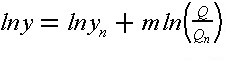 |
| (5.6) | 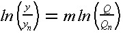 |
Example 5-4: Determination of m for the exponential rule
Figure 5-4: Log-Log Scale Graph of Exponential Rule Example
The empirical cost data from a number of sewage treatment plants are plotted on a log-log scale for ln(Q/Q n ) and ln(y/y n ) and a linear relationship between these logarithmic ratios is shown in Figure 5-4. For (Q/Q n ) = 1 or ln(Q/Q n ) = 0, ln(y/y n ) = 0; and for Q/Q n = 2 or ln(Q/Q n ) = 0.301, ln(y/y n ) = 0.1765. Since m is the slope of the line in the figure, it can be determined from the geometric relation as follows:Example 5-5: Cost exponents for water and wastewater treatment plants [4]For ln(y/y n ) = 0.1765, y/y n = 1.5, while the corresponding value of Q/Q n is 2. In words, for m = 0.585, the cost of a plant increases only 1.5 times when the capacity is doubled .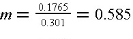
The magnitude of the cost exponent m in the exponential rule provides a simple measure of the economy of scale associated with building extra capacity for future growth and system reliability for the present in the design of treatment plants. When m is small, there is considerable incentive to provide extra capacity since scale economies exist as illustrated in Figure 5-3. When m is close to 1, the cost is directly proportional to the design capacity. The value of m tends to increase as the number of duplicate units in a system increases. The values of m for several types of treatment plants with different plant components derived from statistical correlation of actual construction costs are shown in Table 5-3.
| | ||
| Treatment plant type | Exponent m | Capacity range (millions of gallons per day) |
| | ||
| 1. Water treatment | 0.67 | 1-100 |
| 2. Waste treatment | ||
| Primary with digestion (small) | 0.55 | 0.1-10 |
| Primary with digestion (large) | 0.75 | 0.7-100 |
| Trickling filter | 0.60 | 0.1-20 |
| Activated sludge | 0.77 | 0.1-100 |
| Stabilization ponds | 0.57 | 0.1-100 |
| | ||
| Source: Data are collected from various sources by P.M. Berthouex. See the references in his article for the primary sources. | ||
Example 5-6: Some Historical Cost Data for the Exponential Rule
The exponential rule as represented by Equation (5.4) can be expressed in a different form as:where If m and K are known for a given type of facility, then the cost y for a proposed new facility of specified capacity Q can be readily computed.
| | |||
| Processing unit | Unit of capacity | K Value (1968 $) | m value |
| | |||
| 1. Liquid processing | |||
| Oil separation | mgd | 58,000 | 0.84 |
| Hydroclone degritter | mgd | 3,820 | 0.35 |
| Primary sedimentation | ft 2 | 399 | 0.60 |
| Furial clarifier | ft 2 | 700 | 0.57 |
| Sludge aeration basin | mil. gal. | 170,000 | 0.50 |
| Tickling filter | ft 2 | 21,000 | 0.71 |
| Aerated lagoon basin | mil. gal. | 46,000 | 0.67 |
| Equalization | mil. gal. | 72,000 | 0.52 |
| Neutralization | mgd | 60,000 | 0.70 |
| 2. Sludge handling | |||
| Digestion | ft 3 | 67,500 | 0.59 |
| Vacuum filter | ft 2 | 9,360 | 0.84 |
| Centrifuge | lb dry solids/hr | 318 | 0.81 |
| | |||
| Source: Data are collected from various sources by P.M. Berthouex. See the references in his article for the primary sources. | |||
The estimated values of K and m for various water and sewage treatment plant components are shown in Table 5-4. The K values are based on 1968 dollars. The range of data from which the K and m values are derived in the primary sources should be observed in order to use them in making cost estimates.
As an example, take K = $399 and m = 0.60 for a primary sedimentation component in Table 5-4. For a proposed new plant with the primary sedimentation process having a capacity of 15,000 sq. ft., the estimated cost (in 1968 dollars) is:
y = ($399)(15,000) 0.60 = $128,000.Back to top
5.5 Unit Cost Method of Estimation
If the design technology for a facility has been specified, the project can be decomposed into elements at various levels of detail for the purpose of cost estimation. The unit cost for each element in the bill of quantities must be assessed in order to compute the total construction cost. This concept is applicable to both design estimates and bid estimates, although different elements may be selected in the decomposition.For design estimates, the unit cost method is commonly used when the project is decomposed into elements at various levels of a hierarchy as follows:
- Preliminary Estimates . The project is decomposed into major structural systems or production equipment items, e.g. the entire floor of a building or a cooling system for a processing plant.
- Detailed Estimates . The project is decomposed into components of various major systems, i.e., a single floor panel for a building or a heat exchanger for a cooling system.
- Engineer's Estimates . The project is decomposed into detailed items of various components as warranted by the available cost data. Examples of detailed items are slabs and beams in a floor panel, or the piping and connections for a heat exchanger.
- Subcontractor Quotations . The decomposition of a project into subcontractor items for quotation involves a minimum amount of work for the general contractor. However, the accuracy of the resulting estimate depends on the reliability of the subcontractors since the general contractor selects one among several contractor quotations submitted for each item of subcontracted work.
- Quantity Takeoffs . The decomposition of a project into items of quantities that are measured (or taken off ) from the engineer's plan will result in a procedure similar to that adopted for a detailed estimate or an engineer's estimate by the design professional. The levels of detail may vary according to the desire of the general contractor and the availability of cost data.
- Construction Procedures . If the construction procedure of a proposed project is used as the basis of a cost estimate, the project may be decomposed into items such as labor, material and equipment needed to perform various tasks in the projects.
Simple Unit Cost Formula
Suppose that a project is decomposed into n elements for cost estimation. Let Q i be the quantity of the i th element and u i be the corresponding unit cost. Then, the total cost of the project is given by:| (5.7) |  |
Factored Estimate Formula
A special application of the unit cost method is the "factored estimate" commonly used in process industries. Usually, an industrial process requires several major equipment components such as furnaces, towers drums and pump in a chemical processing plant, plus ancillary items such as piping, valves and electrical elements. The total cost of a project is dominated by the costs of purchasing and installing the major equipment components and their ancillary items. Let C i be the purchase cost of a major equipment component i and f i be a factor accounting for the cost of ancillary items needed for the installation of this equipment component i. Then, the total cost of a project is estimated by:| (5.8) |  |
Formula Based on Labor, Material and Equipment
Consider the simple case for which costs of labor, material and equipment are assigned to all tasks. Suppose that a project is decomposed into n tasks. Let Q i be the quantity of work for task i, M i be the unit material cost of task i, E i be the unit equipment rate for task i, L i be the units of labor required per unit of Q i , and W i be the wage rate associated with L i . In this case, the total cost y is:| (5.9) |  |
Example 5-7: Decomposition of a building foundation into design and construction elements.
The concept of decomposition is illustrated by the example of estimating the costs of a building foundation excluding excavation as shown in Table 5-5 in which the decomposed design elements are shown on horizontal lines and the decomposed contract elements are shown in vertical columns . For a design estimate, the decomposition of the project into footings, foundation walls and elevator pit is preferred since the designer can easily keep track of these design elements; however, for a bid estimate, the decomposition of the project into formwork, reinforcing bars and concrete may be preferred since the contractor can get quotations of such contract items more conveniently from specialty subcontractors.
| | ||||
| Design elements | Contract elements | |||
| | ||||
| Formwork | Rebars | Concrete | Total cost | |
| | ||||
| Footings | $5,000 | $10,000 | $13,000 | $28,000 |
| Footings | 15,000 | 18,000 | 28,000 | 61,000 |
| Footings | 9,000 | 15,000 | 16,000 | 40,000 |
| Total cost | $29,000 | $43,000 | $57,000 | $129,000 |
| | ||||
Example 5-8: Cost estimate using labor, material and equipment rates.
For the given quantities of work Q i for the concrete foundation of a building and the labor, material and equipment rates in Table 5-6, the cost estimate is computed on the basis of Equation (5.9). The result is tabulated in the last column of the same table.
| | |||||||
| Description | Quantity Q i | Material unit cost M i | Equipment unit cost E i | Wage rate W i | Labor input L i | Labor unit cost W i L i | Direct cost Y i |
| | |||||||
| Formwork | 12,000 ft 2 | $0.4/ft 2 | $0.8/ft 2 | $15/hr | 0.2 hr/ft 2 | $3.0/ft 2 | $50,400 |
| Rebars | 4,000 lb | 0.2/lb | 0.3/lb | 15/hr | 0.04 hr/lb | 0.6/lb | 4,440 |
| Concrete | 500 yd 3 | 5.0/yd 3 | 50/yd 3 | 15/hr | 0.8 hr/yd 3 | 12.0/yd 3 | 33,500 |
| Total | $88,300 | ||||||
| | |||||||
5.6 Methods for Allocation of Joint Costs
The principle of allocating joint costs to various elements in a project is often used in cost estimating. Because of the difficulty in establishing casual relationship between each element and its associated cost, the joint costs are often prorated in proportion to the basic costs for various elements.One common application is found in the allocation of field supervision cost among the basic costs of various elements based on labor, material and equipment costs, and the allocation of the general overhead cost to various elements according to the basic and field supervision cost. Suppose that a project is decomposed into n tasks. Let y be the total basic cost for the project and y i be the total basic cost for task i. If F is the total field supervision cost and F i is the proration of that cost to task i, then a typical proportional allocation is:
| (5.10) |  |
| (5.11) |  |
| (5.12) |  |
| (5.13) |  |
Example 5-9: Prorated costs for field supervision and office overhead
If the field supervision cost is $13,245 for the project in Table 5-6 (Example 5-8) with a total direct cost of $88,300, find the prorated field supervision costs for various elements of the project. Furthermore, if the general office overhead charged to the project is 4% of the direct field cost which is the sum of basic costs and field supervision cost, find the prorated general office overhead costs for various elements of the project.For the project, y = $88,300 and F = $13,245. Hence:
z = 13,245 + 88,300 = $101,545The results of the proration of costs to various elements are shown in Table 5-7.
G = (0.04)(101,545) = $4,062
w = 101,545 + 4,062 = $105,607
| | |||||||
| Description | Basic cost y i | Allocated field supervision cost F i | Total field cost z i | Allocated overhead cost G i | Total cost L i | ||
| | |||||||
| Formwork | $50,400 | $7,560 | $57,960 | $2,319 | $60,279 | ||
| Rebars | 4,400 | 660 | 5,060 | 202 | 5,262 | ||
| Concrete | 33,500 | 5,025 | 38,525 | 1,541 | 40,066 | ||
| Total | $88,300 | $13,245 | $101,545 | $4,062 | $105,607 | ||
| | |||||||
Example 5-10: A standard cost report for allocating overhead
The reliance on labor expenses as a means of allocating overhead burdens in typical management accounting systems can be illustrated by the example of a particular product's standard cost sheet. [5] Table 5-8 is an actual product's standard cost sheet of a company following the procedure of using overhead burden rates assessed per direct labor hour . The material and labor costs for manufacturing a type of valve were estimated from engineering studies and from current material and labor prices. These amounts are summarized in Columns 2 and 3 of Table 5-8. The overhead costs shown in Column 4 of Table 5-8 were obtained by allocating the expenses of several departments to the various products manufactured in these departments in proportion to the labor cost. As shown in the last line of the table, the material cost represents 29% of the total cost, while labor costs are 11% of the total cost. The allocated overhead cost constitutes 60% of the total cost. Even though material costs exceed labor costs, only the labor costs are used in allocating overhead. Although this type of allocation method is common in industry, the arbitrary allocation of joint costs introduces unintended cross subsidies among products and may produce adverse consequences on sales and profits. For example, a particular type of part may incur few overhead expenses in practice, but this phenomenon would not be reflected in the standard cost report.
| | ||||
| (1) Material cost | (2) Labor cost | (3) Overhead cost | (4) Total cost | |
| | ||||
| Purchased part | $1.1980 | $1.1980 | ||
| Operation | ||||
| Drill, face, tap (2) | $0.0438 | $0.2404 | $0.2842 | |
| Degrease | 0.0031 | 0.0337 | 0.0368 | |
| Remove burs | 0.0577 | 0.3241 | 0.3818 | |
| Total cost, this item | 1.1980 | 0.1046 | 0.5982 | 1.9008 |
| Other subassemblies | 0.3523 | 0.2994 | 1.8519 | 2.4766 |
| Total cost, subassemblies | 1.5233 | 0.4040 | 2.4501 | 4.3773 |
| Assemble and test | 0.1469 | 0.4987 | 0.6456 | |
| Pack without paper | 0.0234 | 0.1349 | 0.1583 | |
| Total cost, this item | $1.5233 | $0.5743 | $3.0837 | $5.1813 |
| Cost component, % | 29% | 11% | 60% | 100% |
| | ||||
| Source: H. T. Johnson and R. S. Kaplan, Relevance lost: The Rise and Fall of Management Accounting , Harvard Business School Press, Boston. Reprinted with permission. | ||||
Back to top
5.7 Historical Cost Data
Preparing cost estimates normally requires the use of historical data on construction costs. Historical cost data will be useful for cost estimation only if they are collected and organized in a way that is compatible with future applications. Organizations which are engaged in cost estimation continually should keep a file for their own use. The information must be updated with respect to changes that will inevitably occur. The format of cost data, such as unit costs for various items, should be organized according to the current standard of usage in the organization.Construction cost data are published in various forms by a number of organizations. These publications are useful as references for comparison. Basically, the following types of information are available:
- Catalogs of vendors' data on important features and specifications relating to their products for which cost quotations are either published or can be obtained. A major source of vendors ' information for building products is Sweets' Catalog published by McGraw-Hill Information Systems Company.
- Periodicals containing construction cost data and indices. One source of such information is ENR , the McGraw-Hill Construction Weekly, which contains extensive cost data including quarterly cost reports . Cost Engineering , a journal of the American Society of Cost Engineers, also publishes useful cost data periodically.
- Commercial cost reference manuals for estimating guides. An example is the Building Construction Cost Data published annually by R.S. Means Company, Inc., which contains unit prices on building construction items. Dodge Manual for Building Construction , published by McGraw-Hill, provides similar information.
- Digests of actual project costs. The Dodge Digest of Building Costs and Specifications provides descriptions of design features and costs of actual projects by building type. Once a week, ENR publishes the bid prices of a project chosen from all types of construction projects.
Since the future prices of constructed facilities are influenced by many uncertain factors, it is important to recognize that this risk must be borne to some degree by all parties involved, i.e., the owner, the design professionals, the construction contractors, and the financing institution. It is to the best interest of all parties that the risk sharing scheme implicit in the design/construct process adopted by the owner is fully understood by all. When inflation adjustment provisions have very different risk implications to various parties, the price level changes will also be treated differently for various situations. Back to top
5.8 Cost Indices
Since historical cost data are often used in making cost estimates, it is important to note the price level changes over time. Trends in price changes can also serve as a basis for forecasting future costs. The input price indices of labor and/or material reflect the price level changes of such input components of construction; the output price indices, where available, reflect the price level changes of the completed facilities, thus to some degree also measuring the productivity of construction.A price index is a weighted aggregate measure of constant quantities of goods and services selected for the package. The price index at a subsequent year represents a proportionate change in the same weighted aggregate measure because of changes in prices. Let l t be the price index in year t, and l t+1 be the price index in the following year t+1. Then, the percent change in price index for year t+1 is:
| (5.14) |  |
| (5.15) |  |
The best-known indicators of general price changes are the Gross Domestic Product (GDP) deflators compiled periodically by the U.S. Department of Commerce, and the consumer price index (CPI) compiled periodically by the U.S. Department of Labor. They are widely used as broad gauges of the changes in production costs and in consumer prices for essential goods and services. Special price indices related to construction are also collected by industry sources since some input factors for construction and the outputs from construction may disproportionately outpace or fall behind the general price indices. Examples of special price indices for construction input factors are the wholesale Building Material Price and Building Trades Union Wages, both compiled by the U.S. Department of Labor. In addition, the construction cost index and the building cost index are reported periodically in the Engineering News-Record (ENR) . Both ENR cost indices measure the effects of wage rate and material price trends, but they are not adjusted for productivity, efficiency, competitive conditions, or technology changes. Consequently, all these indices measure only the price changes of respective construction input factors as represented by constant quantities of material and/or labor. On the other hand, the price indices of various types of completed facilities reflect the price changes of construction output including all pertinent factors in the construction process. The building construction output indices compiled by Turner Construction Company and Handy-Whitman Utilities are compiled in the U.S. Statistical Abstracts published each year.
Figure 5-7 and Table 5-9 show a variety of United States indices, including the Gross National Product (GNP) price deflator, the ENR building index, the Handy Whitman Utilities Buildings, and the Turner Construction Company Building Cost Index from 1970 to 1998, using 1992 as the base year with an index of 100.
| Year | 1970 | 1975 | 1980 | 1985 | 1990 | 1993 | 1994 | 1995 | 1996 | 1997 | 1998 |
| Turner Construction - Buildings | 28 | 44 | 61 | 83 | 98 | 102 | 105 | 109 | 112 | 117 | 122 |
| ENR - Buildings | 28 | 44 | 68.5 | 85.7 | 95.4 | 105.7 | 109.8 | 109.8 | 113 | 118.7 | 119.7 |
| US Census - Composite | 28 | 44 | 68.6 | 82.9 | 98.5 | 103.7 | 108 | 112.5 | 115 | 118.7 | 122 |
| Handy-Whitman Public Utility | 31 | 54 | 78 | 90 | 101 | 105 | 112 | 115 | 118 | 122 | 123 |
| GNP Deflator | 35 | 49 | 70 | 92 | 94 | 103 | 105 | 108 | 110 | 113 | 114 |
Figure 5-7 Trends for US price indices.
Figure 5-8 Price and cost indices for construction.
Since construction costs vary in different regions of the United States and in all parts of the world, locational indices showing the construction cost at a specific location relative to the national trend are useful for cost estimation. ENR publishes periodically the indices of local construction costs at the major cities in different regions of the United States as percentages of local to national costs.
When the inflation rate is relatively small, i.e., less than 10%, it is convenient to select a single price index to measure the inflationary conditions in construction and thus to deal only with a single set of price change rates in forecasting. Let j t be the price change rate in year t+1 over the price in year t. If the base year is denoted as year 0 (t=0), then the price change rates at years 1,2,...t are j 1 ,j 2 ,...j t , respectively. Let A t be the cost in year t expressed in base-year dollars and A t ' be the cost in year t expressed in then-current dollars. Then:
| (5.16) | 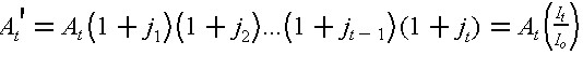 |
| (5.17) |  |
Future forecasts of costs will be uncertain: the actual expenses may be much lower or much higher than those forecasted. This uncertainty arises from technological changes, changes in relative prices, inaccurate forecasts of underlying socioeconomic conditions, analytical errors, and other factors. For the purpose of forecasting, it is often sufficient to project the trend of future prices by using a constant rate j for price changes in each year over a period of t years, then
| (5.18) |  |
| (5.19) | 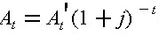 |
| (5.20) |  |
| (5.21) |  |
Example 5-12: Changes in highway and building costs
Table 5-10 shows the change of standard highway costs from 1940 to 1990, and Table 5-11 shows the change of residential building costs from 1970 to 1990. In each case, the rate of cost increase was substantially above the rate of inflation in the decade of the 1970s.. Indeed, the real cost increase between 1970 and 1980 was in excess of three percent per year in both cases. However, these data also show some cause for optimism . For the case of the standard highway, real cost decreases took place in the period from l970 to l990. Unfortunately, comparable indices of outputs are not being compiled on a nationwide basis for other types of construction.
| | ||||
| Year | Standard highway cost (1972=100) | Price deflator (1972=100) | Standard highway real cost (1972=100) | Percentage change per year |
| | ||||
| 1940 | 26 | 29 | 90 | |
| 1950 | 48 | 54 | 89 | -0.1% |
| 1960 | 58 | 69 | 84 | -0.6% |
| 1970 | 91 | 92 | 99 | +1.8% |
| 1980 | 255 | 179 | 143 | +4.4% |
| 1990 | 284 | 247 | 115 | -2.8% |
| | ||||
| Source: Statistical Abstract of the United States. GDP deflator is used for the price deflator index. | ||||
| | ||||
| year | Standard residence cost (1972=100) | Price deflator (1972=100) | Standard residence real cost (1972=100) | Percentage change per year |
| | ||||
| 1970 | 77 | 92 | 74 | |
| 1980 | 203 | 179 | 99 | +3.4% |
| 1990 | 287 | 247 | 116 | +1.7% |
| | ||||
| Source: Statistical Abstract of the United States. GNP deflator is used for the price deflator index. | ||||
Back to top
5.9 Applications of Cost Indices to Estimating
In the screening estimate of a new facility, a single parameter is often used to describe a cost function. For example, the cost of a power plant is a function of electricity generating capacity expressed in megawatts, or the cost of a sewage treatment plant as a function of waste flow expressed in million gallons per day.The general conditions for the application of the single parameter cost function for screening estimates are:
- Exclude special local conditions in historical data
- Determine new facility cost on basis of specified size or capacity (using the methods described in Sections 5.3 to 5.6)
- Adjust for inflation index
- Adjust for local index of construction costs
- Adjust for different regulatory constraints
- Adjust for local factors for the new facility
Example 5-13: Screening estimate for a refinery
The total construction cost of a refinery with a production capacity of 200,000 bbl/day in Gary, Indiana, completed in 2001 was $100 million. It is proposed that a similar refinery with a production capacity of 300,000 bbl/day be built in Los Angeles, California, for completion in 2003. For the additional information given below, make an order of magnitude estimate of the cost of the proposed plant.Example 5-14: Conceptual estimate for a chemical processing plantOn the basis of the above conditions, the estimate for the new project may be obtained as follows:
- In the total construction cost for the Gary, Indiana, plant, there was an item of $5 million for site preparation which is not typical for other plants.
- The variation of sizes of the refineries can be approximated by the exponential rule, Equation (5.4), with m = 0.6.
- The inflation rate is expected to be 8% per year from 1999 to 2003.
- The location index was 0.92 for Gary, Indiana and 1.14 for Los Angeles in 1999. These indices are deemed to be appropriate for adjusting the costs between these two cities.
- New air pollution equipment for the LA plant costs $7 million in 2003 dollars (not required in the Gary plant).
- The contingency cost due to inclement weather delay will be reduced by the amount of 1% of total construction cost because of the favorable climate in LA (compared to Gary).
Since there is no adjustment for the cost of construction financing, the order of magnitude estimate for the new project is $209.5 million.
- Typical cost excluding special item at Gary, IN is
$100 million - $5 million = $ 95 million- Adjustment for capacity based on the exponential law yields
($95)(300,000/200,000) 0.6 = (95)(1.5) 0.6 = $121.2 million- Adjustment for inflation leads to the cost in 2003 dollars as
($121.2)(1.08) 4 = $164.6 million- Adjustment for location index gives
($164.6)(1.14/0.92) = $204.6 million- Adjustment for new pollution equipment at the LA plant gives
$204.6 + $7 = $211.6 million- Reduction in contingency cost yields
($211.6)(1-0.01) = $209.5 million
In making a preliminary estimate of a chemical processing plant, several major types of equipment are the most significant parameters in affecting the installation cost. The cost of piping and other ancillary items for each type of equipment can often be expressed as a percentage of that type of equipment for a given capacity. The standard costs for the major equipment types for two plants with different daily production capacities are as shown in Table 5-12. It has been established that the installation cost of all equipment for a plant with daily production capacity between 100,000 bbl and 400,000 bbl can best be estimated by using linear interpolation of the standard data.Back to top
TABLE 5-12 Cost Data for Equipment and Ancillary Items Equipment
typeEquipment Cost ($1000) Cost of ancillary items
as % of equipment cost ($1000)100,000 bbl 400,000 bbl 100,000 bbl 400,000 bbl Furnace 3,000 10,000 40% 30% Tower 2,000 6,000 45% 35% Drum 1,500 5,000 50% 40% Pump, etc. 1,000 4,000 60% 50% A new chemical processing plant with a daily production capacity of 200,000 bbl is to be constructed in Memphis, TN in four years. Determine the total preliminary cost estimate of the plant including the building and the equipment on the following basis:
The solution of this problem can be carried out according to the steps as outlined in the problem statement:
- The installation cost for equipment was based on linear interpolation from Table 5-12, and adjusted for inflation for the intervening four years. We expect inflation in the four years to be similar to the period 1990-1994 and we will use the GNP Deflator index.
- The location index for equipment installation is 0.95 for Memphis, TN, in comparison with the standard cost.
- An additional cost of $500,000 was required for the local conditions in Memphis, TN.
- The costs of the equipment and ancillary items for a plant with a capacity of 200,000 bbl can be estimated by linear interpolation of the data in Table 5-12, and the results are shown in Table 5-13.
TABLE 5-13 Results of Linear Interpolation for an Estimation Example Equipment
typeEquipment Cost
(in $1,000)Percentage for
ancillary itemsFurnace $3,000 + (1/3)($10,000-$3,000) = $5,333 40% - (1/3)(40%-30%) = 37% Tower $2,000 + (1/3)($6,000-$2,000) = $3,333 45% - (1/3)(45%-35%) = 42% Drum $1,500 + (1/3)($5,000-$1,500) = $2,667 50% - (1/3)(50%-40%) = 47% Pumps, etc. $1,000 + (1/3)($4,000-$1,000) = $2,000 60% - (1/3)(60%-50%) = 57% Hence, the total project cost in thousands of current dollars is given by Equation (5.8) as:
($5,333)(1.37) + ($3,333)(1.42) +($2,667)(1.47) + ($2,000)(1.57) =
= $2,307 + $4,733 + $3,920 + $3,140 = $ 19,000- The corresponding cost in thousands of four year in the future dollars using Equation (5.16) and Table 5-9 is:
($19,100)(105/94) = $21,335- The total cost of the project after adjustment for location is
(0.95)($21,335,000) + $500,000$20,800,000
5.10 Estimate Based on Engineer's List of Quantities
The engineer's estimate is based on a list of items and the associated quantities from which the total construction cost is derived. This same list is also made available to the bidders if unit prices of the items on the list are also solicited from the bidders. Thus, the itemized costs submitted by the winning contractor may be used as the starting point for budget control.In general, the progress payments to the contractor are based on the units of work completed and the corresponding unit prices of the work items on the list. Hence, the estimate based on the engineers' list of quanitities for various work items essentially defines the level of detail to which subsequent measures of progress for the project will be made.
Example 5-15: Bid estimate based on engineer's list of quantities
Using the unit prices in the bid of contractor 1 for the quantitites specified by the engineer in Table 5-2 (Example 5-3), we can compute the total bid price of contractor 1 for the roadway project. The itemized costs for various work items as well as the total bid price are shown in Table 5-14.
| Items | Unit | Quantity | Unit price | Item cost |
| Mobilization | ls | 1 | 115,000 | 115,000 |
| Removal, berm | lf | 8,020 | 1.00 | 8.020 |
| Finish subgrade | sy | 1,207,500 | 0.50 | 603,750 |
| Surface ditches | lf | 525 | 2.00 | 1,050 |
| Excavation structures | cy | 7,000 | 3.00 | 21,000 |
| Base course, untreated, 3/4'' | ton | 362,200 | 4.50 | 1,629,900 |
| Lean concrete, 4'' thick | sy | 820,310 | 3.10 | 2,542,961 |
| PCC, pavement, 10'' thick | sy | 76,010 | 10.90 | 7,695,509 |
| Concrete, ci AA (AE) | ls | 1 | 200,000 | 200,000 |
| Small structure | cy | 50 | 500 | 25,000 |
| Barrier, precast | lf | 7,920 | 15.00 | 118,800 |
| Flatwork, 4'' thick | sy | 7,410 | 10.00 | 74,100 |
| 10'' thick | sy | 4,241 | 20.00 | 84,820 |
| Slope protection | sy | 2,104 | 25.00 | 52,600 |
| Metal, end section, 15'' | ea | 39 | 100 | 3,900 |
| 18'' | ea | 3 | 150 | 450 |
| Post, right-of-way, modification | lf | 4,700 | 3.00 | 14,100 |
| Salvage and relay pipe | lf | 1,680 | 5.00 | 8,400 |
| Loose riprap | cy | 32 | 40.00 | 1,280 |
| Braced posts | ea | 54 | 100 | 5,400 |
| Delineators, type I | lb | 1,330 | 12.00 | 15,960 |
| type II | ea | 140 | 15.00 | 2,100 |
| Constructive signs fixed | sf | 52,600 | 0.10 | 5,260 |
| Barricades, type III | lf | 29,500 | 0.20 | 5,900 |
| Warning lights | day | 6,300 | 0.10 | 630 |
| Pavement marking, epoxy material | ||||
| Black | gal | 475 | 90.00 | 42,750 |
| Yellow | gal | 740 | 90.00 | 66,600 |
| White | gal | 985 | 90.00 | 88,650 |
| Plowable, one-way white | ea | 342 | 50.00 | 17,100 |
| Topsoil, contractor furnished | cy | 260 | 10.00 | 2,600 |
| Seedling, method A | acr | 103 | 150 | 15,450 |
| Excelsior blanket | sy | 500 | 2.00 | 1,000 |
| Corrugated, metal pipe, 18'' | lf | 580 | 20.00 | 11,600 |
| Polyethylene pipe, 12'' | lf | 2,250 | 15.00 | 33,750 |
| Catch basin grate and frame | ea | 35 | 350 | 12,250 |
| Equal opportunity training | hr | 18,000 | 0.80 | 14,400 |
| Granular backfill borrow | cy | 274 | 10.00 | 2,740 |
| Drill caisson, 2'x6'' | lf | 722 | 100 | 72,200 |
| Flagging | hr | 20,000 | 8.25 | 165,000 |
| Prestressed concrete member | ||||
| type IV, 141'x4'' | ea | 7 | 12,000 | 84,000 |
| 132'x4'' | ea | 6 | 11,000 | 66,000 |
| Reinforced steel | lb | 6,300 | 0.60 | 3,780 |
| Epoxy coated | lb | 122,241 | 0.55 | 67,232.55 |
| Structural steel | ls | 1 | 5,000 | 5,000 |
| Sign, covering | sf | 16 | 10.00 | 160 |
| type C-2 wood post | sf | 98 | 15.00 | 1,470 |
| 24'' | ea | 3 | 100 | 300 |
| 30'' | ea | 2 | 100 | 200 |
| 48'' | ea | 11 | 200 | 2,200 |
| Auxiliary | sf | 61 | 15.00 | 915 |
| Steel post, 48''x60'' | ea | 11 | 500 | 5,500 |
| type 3, wood post | sf | 669 | 15.00 | 10,035 |
| 24'' | ea | 23 | 100 | 2,300 |
| 30'' | ea | 1 | 100 | 100 |
| 36'' | ea | 12 | 150 | 1,800 |
| 42''x60'' | ea | 8 | 150 | 1,200 |
| 48'' | ea | 7 | 200 | 1,400 |
| Auxiliary | sf | 135 | 15.00 | 2,025 |
| Steel post | sf | 1,610 | 40.00 | 64,400 |
| 12''x36'' | ea | 28 | 100 | 2,800 |
| Foundation, concrete | ea | 60 | 300 | 18,000 |
| Barricade, 48''x42'' | ea | 40 | 100 | 4,000 |
| Wood post, road closed | lf | 100 | 30.00 | 3,000 |
| Total | $14,129,797.55 | |||
Back to top
5.11 Allocation of Construction Costs Over Time
Since construction costs are incurred over the entire construction phase of a project, it is often necessary to determine the amounts to be spent in various periods to derive the cash flow profile, especially for large projects with long durations. Consequently, it is important to examine the percentage of work expected to be completed at various time periods to which the costs would be charged. More accurate estimates may be accomplished once the project is scheduled as described in Chapter 10, but some rough estimate of the cash flow may be required prior to this time.Consider the basic problem in determining the percentage of work completed during construction. One common method of estimating percentage of completion is based on the amount of money spent relative to the total amount budgeted for the entire project. This method has the obvious drawback in assuming that the amount of money spent has been used efficiently for production. A more reliable method is based on the concept of value of work completed which is defined as the product of the budgeted labor hours per unit of production and the actual number of production units completed, and is expressed in budgeted labor hours for the work completed. Then, the percentage of completion at any stage is the ratio of the value of work completed to date and the value of work to be completed for the entire project. Regardless of the method of measurement, it is informative to understand the trend of work progress during construction for evaluation and control.
In general, the work on a construction project progresses gradually from the time of mobilization until it reaches a plateau; then the work slows down gradually and finally stops at the time of completion. The rate of work done during various time periods (expressed in the percentage of project cost per unit time) is shown schematically in Figure 5-9 in which ten time periods have been assumed. The solid line A represents the case in which the rate of work is zero at time t = 0 and increases linearly to 12.5% of project cost at t = 2, while the rate begins to decrease from 12.5% at t = 8 to 0% at t = 10. The dotted line B represents the case of rapid mobilization by reaching 12.5% of project cost at t = 1 while beginning to decrease from 12.5% at t = 7 to 0% at t = 10. The dash line C represents the case of slow mobilization by reaching 12.5% of project cost at t = 3 while beginning to decrease from 12.5% at t = 9 to 0% at t = 10.
Figure 5-9: Rate of Work Progress over Project Time
The value of work completed at a given time (expressed as a cumulative percentage of project cost) is shown schematically in Figure 5-10. In each case (A, B or C), the value of work completed can be represented by an "S-shaped" curve. The effects of rapid mobilization and slow mobilization are indicated by the positions of curves B and C relative to curve A, respectively.
Figure 5-10: Value of Work Completed over Project Time
While the curves shown in Figures 5-9 and 5-10 represent highly idealized cases, they do suggest the latitude for adjusting the schedules for various activities in a project. While the rate of work progress may be changed quite drastically within a single period, such as the change from rapid mobilization to a slow mobilization in periods 1, 2 and 3 in Figure 5-9, the effect on the value of work completed over time will diminish in significance as indicated by the cumulative percentages for later periods in Figure 5-10. Thus, adjustment of the scheduling of some activities may improve the utilization of labor, material and equipment, and any delay caused by such adjustments for individual activities is not likely to cause problems for the eventual progress toward the completion of a project.
In addition to the speed of resource mobilization, another important consideration is the overall duration of a project and the amount of resources applied. Various strategies may be applied to shorten the overall duration of a project such as overlapping design and construction activities (as described in Chapter 2) or increasing the peak amounts of labor and equipment working on a site. However, spatial, managerial and technical factors will typically place a minimum limit on the project duration or cause costs to escalate with shorter durations.
Example 5-16: Calculation of Value of Work Completed
From the area of work progress in Figure 5-9, the value of work completed at any point in Figure 5-10 can be derived by noting the area under the curve up to that point in Figure 5-9. The result for t = 0 through t = 10 is shown in Table 5-15 and plotted in Figure 5-10.
| | |||
| Time | Case A | Case B | Case C |
| | |||
| 1 | 3.1% | 6.2% | 2.1% |
| 2 | 12.5 | 18.7 | 8.3 |
| 3 | 25.0 | 31.2 | 18.8 |
| 4 | 37.5 | 43.7 | 31.3 |
| 5 | 50.0 | 56.2 | 43.8 |
| 6 | 62.5 | 68.7 | 56.3 |
| 7 | 75.0 | 81.2 | 68.8 |
| 8 | 87.5 | 91.7 | 81.9 |
| 9 | 96.9 | 97.9 | 93.8 |
| 10 | 100.0 | 100.0 | 100.0 |
| | |||
Back to top
5.12 Computer Aided Cost Estimation
Numerous computer aided cost estimation software systems are now available. These range in sophistication from simple spreadsheet calculation software to integrated systems involving design and price negotiation over the Internet. While this software involves costs for purchase, maintenance, training and computer hardware, some significant efficiencies often result. In particular, cost estimates may be prepared more rapidly and with less effort.Some of the common features of computer aided cost estimation software include:
- Databases for unit cost items such as worker wage rates, equipment rental or material prices. These databases can be used for any cost estimate required. If these rates change, cost estimates can be rapidly re-computed after the databases are updated.
- Databases of expected productivity for different components types, equiptment and construction processes.
- Import utilities from computer aided design software for automatic quantity-take-off of components. Alternatively, special user interfaces may exist to enter geometric descriptions of components to allow automatic quantity-take-off.
- Export utilities to send estimates to cost control and scheduling software. This is very helpful to begin the management of costs during construction.
- Version control to allow simulation of different construction processes or design changes for the purpose of tracking changes in expected costs.
- Provisions for manual review, over-ride and editing of any cost element resulting from the cost estimation system
- Flexible reporting formats, including provisions for electronic reporting rather than simply printing cost estimates on paper.
- Archives of past projects to allow rapid cost-estimate updating or modification for similar designs.
- If a similar design has already been estimated or exists in the company archive, the old project information is retreived.
- A cost engineer modifies, add or deletes components in the project information set. If a similar project exists, many of the components may have few or no updates, thereby saving time.
- A cost estimate is calculated using the unit cost method of estimation. Productivities and unit prices are retrieved from the system databases. Thus, the latest price information is used for the cost estimate.
- The cost estimation is summarized and reviewed for any errors.
5.13 Estimation of Operating Costs
In order to analyze the life cycle costs of a proposed facility, it is necessary to estimate the operation and maintenance costs over time after the start up of the facility. The stream of operating costs over the life of the facility depends upon subsequent maintenance policies and facility use. In particular, the magnitude of routine maintenance costs will be reduced if the facility undergoes periodic repairs and rehabilitation at periodic intervals.Since the tradeoff between the capital cost and the operating cost is an essential part of the economic evaluation of a facility, the operating cost is viewed not as a separate entity, but as a part of the larger parcel of life cycle cost at the planning and design stage. The techniques of estimating life cycle costs are similar to those used for estimating capital costs, including empirical cost functions and the unit cost method of estimating the labor, material and equipment costs. However, it is the interaction of the operating and capital costs which deserve special attention.
As suggested earlier in the discussion of the exponential rule for estimating, the value of the cost exponent may influence the decision whether extra capacity should be built to accommodate future growth. Similarly, the economy of scale may also influence the decision on rehabilitation at a given time. As the rehabilitation work becomes extensive, it becomes a capital project with all the implications of its own life cycle. Hence, the cost estimation of a rehabilitation project may also involve capital and operating costs.
While deferring the discussion of the economic evaluation of constructed facilities to Chapter 6, it is sufficient to point out that the stream of operating costs over time represents a series of costs at different time periods which have different values with respect to the present. Consequently, the cost data at different time periods must be converted to a common base line if meaningful comparison is desired.
Example 5-17: Maintenance cost on a roadway [6]
Maintenance costs for constructed roadways tend to increase with both age and use of the facility. As an example, the following empirical model was estimated for maintenance expenditures on sections of the Ohio Turnpike:
C = 596 + 0.0019 V + 21.7 Awhere C is the annual cost of routine maintenance per lane-mile (in 1967 dollars), V is the volume of traffic on the roadway (measured in equivalent standard axle loads, ESAL, so that a heavy truck is represented as equivalent to many automobiles), and A is the age of the pavement in years since the last resurfacing. According to this model, routine maintenance costs will increase each year as the pavement service deteriorates. In addition, maintenance costs increase with additional pavement stress due to increased traffic or to heavier axle loads, as reflected in the variable V.
For example, for V = 500,300 ESAL and A = 5 years, the annual cost of routine maintenance per lane-mile is estimated to be:
C = 596 + (0.0019)(500,300) + (21.7)(5)Example 5-18: Time stream of costs over the life of a roadway [7]
= 596 + 950.5 + 108.5 = 1,655 (in 1967 dollars)
The time stream of costs over the life of a roadway depends upon the intervals at which rehabilitation is carried out. If the rehabilitation strategy and the traffic are known, the time stream of costs can be estimated.
Using a life cycle model which predicts the economic life of highway pavement on the basis of the effects of traffic and other factors, an optimal schedule for rehabilitation can be developed. For example, a time stream of costs and resurfacing projects for one pavement section is shown in Figure 5-11. As described in the previous example, the routine maintenance costs increase as the pavement ages, but decline after each new resurfacing. As the pavement continues to age, resurfacing becomes more frequent until the roadway is completely reconstructed at the end of 35 years.
Figure 5-11: Time Stream of Costs over the Life of a Highway Pavement
5.14 References
- Ahuja, H.N. and W.J. Campbell, Estimating: From Concept to Completion , Prentice-Hall, Inc., Englewood Cliffs, NJ, 1987.
- Clark, F.D., and A.B. Lorenzoni, Applied Cost Engineering , Marcel Dekker, Inc., New York, 1978.
- Clark, J.E., Structural Concrete Cost Estimating , McGraw-Hill, Inc., New York, 1983.
- Diekmann, J.R., "Probabilistic Estimating: Mathematics and Applications," ASCE Journal of Construction Engineering and Management , Vol. 109, 1983, pp. 297-308.
- Humphreys, K.K. (ed.) Project and Cost Engineers' Handbook (sponsored by American Association of Cost Engineers), 2nd Ed., Marcel Dekker, Inc., New York, 1984.
- Maevis, A.C., "Construction Cost Control by the Owners," ASCE Journal of the Construction Division , Vol. 106, 1980, pp. 435-446.
- Wohl, M. and C. Hendrickson, Transportation Investment and Pricing Principles, John Wiley & Sons, New York, 1984.
5.15 Problems
- Suppose that the grouting method described in Example 5-2 is used to provide a grouting seal beneath another landfill of 12 acres. The grout line is expected to be between 4.5 and 5.5 feet thickness. The voids in the soil layer are between 25% to 35%. Using the same unit cost data (in 1978 dollars), find the range of costs in a screening estimate for the grouting project.
- To avoid submerging part of U.S. Route 40 south and east of Salt Lake City due to the construction of the Jardinal Dam and Reservoir, 22 miles of highway were relocated to the west around the site of the future reservoir. Three separate contracts were let, including one covering 10 miles of the work which had an engineer's estimate of $34,095,545. The bids were submitted on July 21, 1987 and the completion date of the project under the contract was August 15, 1989. (See ENR , October 8, 1987, p. 34). The three lowest bids were:
Find the percentage of each of these bidders below the engineer's cost estimate.1) W.W. Clyde & Co., Springville, Utah
2) Sletten Construction company, Great Falls, Montana
3) Gilbert Western Corporation, Salt Lake city, Utah$21,384,919
$26,701,018
$30,896,203
- In making a screening estimate of an industrial plant for the production of batteries, an empirical formula based on data of a similar buildings completed before 1987 was proposed:
C = (16,000)(Q + 50,000) 1/2
where Q is the daily production capacity of batteries and C is the cost of the building in 1987 dollars. If a similar plant is planned for a daily production capacity of 200,000 batteries, find the screening estimate of the building in 1987 dollars.
- For the cost factor K = $46,000 (in 1968 dollars) and m = 0.67 for an aerated lagoon basin of a water treatment plant in Table 5-4 (Example 5-6), find the estimated cost of a proposed new plant with a similar treatment process having a capacity of 480 million gallons (in 1968 dollars). If another new plant was estimated to cost $160,000 by using the same exponential rule, what would be the proposed capacity of that plant?
- Using the cost data in Figure 5-5 (Example 5-11), find the total cost including overhead and profit of excavating 90,000 cu.yd. of bulk material using a backhoe of 1.5 cu.yd. capacity for a detailed estimate. Assume that the excavated material will be loaded onto trucks for disposal.
- The basic costs (labor, material and equipment) for various elements of a construction project are given as follows:
Assuming that field supervision cost is 10% of the basic cost, and the general office overhead is 5% of the direct costs (sum of the basic costs and field supervision cost), find the prorated field supervision costs, general office overhead costs and total costs for the various elements of the project.Excavation
Subgrade
Base course
Concrete pavement
Total$240,000
$100,000
$420,000
$640,000
$1,400,000
- In making a preliminary estimate of a chemical processing plant, several major types of equipment are the most significant components in affecting the installation cost. The cost of piping and other ancillary items for each type of equipment can often be expressed as a percentage of that type of equipment for a given capacity. The standard costs for the major equipment types for two plants with different daily production capacities are as shown in Table 5-16. It has been established that the installation cost of all equipment for a plant with daily production capacity between 150,000 bbl and 600,000 bbl can best be estimated by using liner interpolation of the standard data. A new chemical processing plant with a daily production capacity of 400,000 bbl is being planned. Assuming that all other factors remain the same, estimate the cost of the new plant.
Table 5-16 Equipment type Equipment cost ($1,000) Factor for ancillary items 150,000 bbl 600,000 bbl 150,000 bbl 600,000 bbl Furnace
Tower
Drum
Pumps, etc.$3,000
2,000
1,500
1,000$10,000
6,000
5,000
4,0000.32
0.42
0.42
0.540.24
0.36
0.32
0.42
- The total construction cost of a refinery with a production capacity of 100,000 bbl/day in Caracas, Venezuela, completed in 1977 was $40 million. It was proposed that a similar refinery with a production capacity of $160,000 bbl/day be built in New Orleans, LA for completion in 1980. For the additional information given below, make a screening estimate of the cost of the proposed plant.
- In the total construction cost for the Caracus, Venezuela plant, there was an item of $2 million for site preparation and travel which is not typical for similar plants.
- The variation of sizes of the refineries can be approximated by the exponential law with m = 0.6.
- The inflation rate in U.S. dollars was approximately 9% per year from 1977 to 1980.
- An adjustment factor of 1.40 was suggested for the project to account for the increase of labor cost from Caracas, Venezuela to New Orleans, LA.
- New air pollution equipment for the New Orleans, LA plant cost $4 million in 1980 dollars (not required for the Caracas plant).
- The site condition at New Orleans required special piling foundation which cost $2 million in 1980 dollars.
- The total cost of a sewage treatment plant with a capacity of 50 million gallons per day completed 1981 for a new town in Colorado was $4.5 million. It was proposed that a similar treatment plant with a capacity of 80 million gallons per day be built in another town in New Jersey for completion in 1985. For additional information given below, make a screening estimate of the cost of the proposed plant.
- In the total construction cost in Colorado, an item of $300,000 for site preparation is not typical for similar plants.
- The variation of sizes for this type of treatment plants can be approximated by the exponential law with m = 0.5.
- The inflation rate was approximately 5% per year from 1981 to 1985.
- The locational indices of Colorado and New Jersey areas are 0.95 and 1.10, respectively, against the national average of 1.00.
- The installation of a special equipment to satisfy the new environmental standard cost an extra $200,000 in 1985 dollar for the New Jersey plant.
- The site condition in New Jersey required special foundation which cost $500,00 in 1985 dollars.
- Using the ENR building cost index, estimate the 1985 cost of the grouting seal on a landfill described in Example 5-2, including the most likely estimate and the range of possible cost.
- Using the unit prices in the bid of contractor 2 for the quantitites specified by the engineer in Table 5-2 (Example 5-3), compute the total bid price of contractor 2 for the roadway project including the expenditure on each item of work.
- The rate of work progress in percent of completion per period of a construction project is shown in Figure 5-12 in which 13 time periods have been assumed. The cases A, B and C represent the normal mobilization time, rapid mobilization and slow mobilization for the project, respectively. Calculate the value of work completed in cumulative percentage for periods 1 through 13 for each of the cases A, B and C. Also plot the volume of work completed versus time for these cases.
Figure 5-12
- The rate of work progress in percent of completion per period of a construction project is shown in Figure 5-13 in which 10 time periods have been assumed. The cases A, B and C represent the rapid mobilization time, normal mobilization and slow mobilization for the project, respectively. Calculate the value of work completed in cumulative percentage for periods 1 through 10 for each of the cases A, B and C. Also plot the volume of work completed versus time for these cases.

Figure 5-13
- Suppose that the empirical model for estimating annual cost of routine maintenance in Example 5-17 is applicable to sections of the Pennsylvania Turnpike in 1985 if the ENR building cost index is applied to inflate the 1967 dollars. Estimate the annual cost of maintenance per lane-mile of the tunrpike for which the traffic volume on the roadway is 750,000 ESAL and the age of the pavement is 4 years in 1985.
- The initial construction cost for a electric rower line is known to be a function of the cross-sectional area A (in cm 2 ) and the length L (in kilometers). Let C 1 be the unit cost of construction (in dollars per cm 3 ). Then, the initial construction cost P (in dollars) is given by
P = C 1 AL(10 5 )
The annual operating cost of the power line is assumed to be measured by the power loss. The power loss S (in kwh) is known to be
where J is the electric current in amperes, R is the resistivity in ohm-centimeters. Let C 2 be the unit operating cost (in dollars per kwh). Then, the annual operating cost U (in dollars) is given by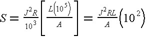
Suppose that the power line is expected to last n years and the life cycle cost T of the power line is equal to: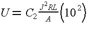
T = P + UK
where K is a discount factor depending on the useful life cycle n and the discount rate i (to be explained in Chapter 6). In designing the power line, all quantitites are assumed to be known except A which is to be determined. If the owner wants to minimize the life cycle cost, find the best cross-sectional area A in terms of the known quantities.
5.16 Footnotes
1. This example was adapted with permission from a paper, "Forecasting Industry Resources," presented by A.R. Crosby at the Institution of Chemical Engineers in London, November 4, 1981. (Back)2. This example is adapted from a cost estimate in A.L. Tolman, A.P. Ballestero, W.W. Beck and G.H. Emrich, Guidance Manual for Minimizing Pollution from Waste Disposal Sites, Municipal Environmental Research Laboratory, U.S. Environmental Protection Agency, Cincinatti, Ohio, 1978. (Back)
3. See "Utah Interstate Forges On," ENR , July 2, 1987, p. 39.(Back)
4. This and the next example have been adapted from P.M. Berthouex, "Evaluating Economy of Scale," Journal of the Water Pollution Control Federation , Vol. 44, No. 11, November 1972, pp. 2111-2118. (Back)
5. See H.T. Johnson and R.S. Kaplan, Relevance Lost: The Rise and Fall of Management Accounting, Harvard Business School Press, Boston, MA 1987, p. 185. (Back)
6. This example is adapted from McNeil, S. and C. Hendrickson, "A Statistical Model of Pavement Maintenance Expenditure," Transportation Research Record No. 846, 1982, pp. 71-76. (Back)
7. This example is adapted from S. McNeil, Three Statistical Models of Road Management Based on Turnpike Data, M.S. Thesis, Carnegie-Mellon University, Pittsburgh, PA, 1981. (Back)
| Previous Chapter | Table of Contents | Next Chapter |
EAN: 2147483647
Pages: 18