Hack 42 Create Ranges That Expand and Contract

   

If you need to constantly update and add to your data, or if you work with charts and PivotTables, you'll want to create dynamic named ranges, which expand and contract relative to your data .

To understand how dynamic named ranges function, first you should familiarize yourself with Excels OFFSET function (if you haven't already). The OFFSET function is one of Excel's Lookup and Reference functions.

We'll start off with the simplest of dynamic named ranges, one that will expand down a single column, but only as far as there are entries in that column. For example, if column A contains 10 continuous rows of data, your dynamic named range will incorporate the range A1:A10. Follow these steps to create a basic dynamic named range.

Select Insert Name Define, and in the Names in Workbook: box, type MyRange . In the Refers To: box, type the following:

 =OFFSET($A,0,0,COUNTA($A:$A0),1) 

Now click Add, then OK.

When defining the range for COUNTA , resist the temptation to include an entire column of data so that you do not force the COUNTA function to count potentially thousands of unnecessary cells .

Now, provided that you have some data in column A, this named range will incorporate all the data in continuous rows, starting from cell A1. If you want to check a dynamic named range, you can do so in a few ways.

Unfortunately, dynamic named ranges are not available via the standard Name box, immediately to the left of the Formula bar. Despite this, you can click the Name box, type the name MyRange , and press Enter. Excel automatically will select the range. Of course, you also can use the Go To... dialog by selecting Edit Go To... (Ctrl/ -G) and typing MyRange in the Reference: box, then clicking OK.

The dynamic named range you created in the previous example nests the COUNTA function as the Height argument in the OFFSET function.

Remember that COUNTA will count all nonblank cells. Be aware that this also will include formulas you have in those cells, which might be returning empty text ("").

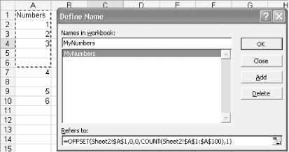
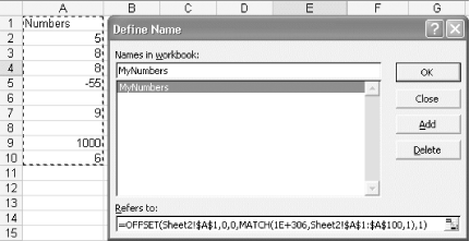
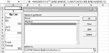
If you have a list that contained numeric data only, and at the end of this list you want to store text, but don't want this text included as part of your dynamic named range, you could replace the COUNTA function with Excel's standard COUNT function. COUNT counts only cells containing numeric data.

In this next example, you will use the dynamic named range to define a table of data that you want to be dynamic. To do this, type the following function into the Refers To: box:

 =OFFSET($A,0,0,COUNTA($A:$A0),COUNTA(:)) 

Here, the dynamic named range will expand down as many entries as there are in column A, and across as many rows as there are headings in row 1. If you are sure the number of columns for your table of data will remain stable, you can replace the second COUNTA function with a fixed number such as 10.

The only problem with using a dynamic named range for a table of data is that it assumes column A will set the maximum length for the table. In most cases, this probably will be true; however, sometimes the longest column might be another column on the spreadsheet.

To overcome this potential problem, you can use Excel's MAX function, which returns the highest number in a range of cells. As an example, set up a table in a manner similar to the one shown in Figure 3-4.

Figure 3-4. Dynamic table of data and the Define Name dialog

Use row 1 to store a number of COUNTA functions that are referencing down the column and, thus, returning the number of entries in each column. Use the MAX function for the Height argument in the OFFSET function. This ensures that the dynamic named range for the table always will expand down as far as the longest column in the table. You can, of course, hide row 1, as there is no need for a user to see it.

In all these examples, you assumed your data will always be in continuous rows without blank cells in between. Although this is the correct way to set up a list or a table of data, sometimes you have no control over this.

In the next example, the list of numbers in column A also contains blank cells. This means that if you try to use the COUNT or COUNTA function, the dynamic named range will fall short of the real last cell containing any data. For example, consider Figure 3-5.

Figure 3-5. Range of numbers and Define Name dialog

In this case, although the last number in the range is actually in row 10, the dynamic range is expanding down to row 6. This is because you used the COUNT function to count from A1 to A100. Only six numeric entries are in the list, so the range expands down only six rows.

To overcome this problem, use Excel's MATCH function. The MATCH function is used to return the relative position of an item in an array that matches a specified value in a specified order. For example, if you use this MATCH function:

 =MATCH(6,$A:$A0,0) 

on the same set of numbers as shown in Figure 3-5, the MATCH function will return the number 10 , representing row 10 in column A. It returns 10 because you told the function to find the number 6 in the range A1:A100.

Obviously, when using the MATCH function as part of a dynamic named range, the last number in the range probably is not known in advance. Therefore, you need to tell the MATCH function to try and locate a ridiculously high number in the range that would never exist and to swap the last argument for the MATCH function from to 1.

In the previous example, you told MATCH to find the exact number 6, nothing less and nothing more. Replacing with 1 tells MATCH to locate the largest value that is less than or equal to that value.

To do this, use this formula:

 =MATCH(1E+306,$A:$A0,1) 

To create a dynamic named range that will expand down to the last row that contains a number (regardless of the blank cells in between), type this formula into the Refers To: box of the Define Name dialog, as illustrated in Figure 3-6:

Figure 3-6. A dynamic range extending to the last numeric entry

 =OFFSET(Sheet2!$A,0,0,MATCH(1E+306,Sheet2!$A:$A0,1),1) 

The next logical type of dynamic named range that would flow on from this is one that will expand down to the last text entry, regardless of any blank cells in the list or table.

To do this, replace the MATCH function with the following:

 MATCH("*",$A:$A0,-1) 

This always will return the row number for the last text entry in range $A$1:$A$100.

Now that you know how to do this for numeric entries and text entries, it is only logical that you need to somehow define a dynamic named range that will look past blank cells in a list that contains both text and numeric data.

To do this, first insert two blank rows above your list by selecting rows 1 and 2 and then selecting Insert Row. In the first row (row 1), add this function:

 =MAX(MATCH"*",$A:$A0,-1),MATCH(1E+306,$A:$A0,1)) 

In the cell immediately below this, place the number 1 . The cell below this must contain a text heading for your list. You added the number 1 so that the second MATCH function does not return #N/A when or if there are no numbers in A3:A100. The second MATCH function will always find text because you have a heading.

Name cell A1 MaxRow and select Insert Name Define, give the dynamic range a name, such as MyList , and in the Refers To: box, as shown in Figure 3-7, type the following:

Figure 3-7. Dynamic list for numeric and text entries containing blanks

 =OFFSET(Sheet2!$A,0,0,MaxRow,1) 

The following list outlines other types of dynamic named ranges you might find useful. For all of these examples, you will need to fill column A with a mix of text and numeric entries. To do this, select Insert Name Define, and in the Names in Workbook: box, type any one-word name (for instance, MyRange ). The only part that will change is the formula you place in the Refers To: box.

Expand down as many rows as there are numeric entries

In the Refers To: box, type the following:

 =OFFSET($A,0,0,COUNT($A:$A),1) 

Expand down as many rows as there are numeric and text entries

In the Refers To: box, type the following:

 =OFFSET($A,0,0,COUNTA($A:$A),1) 

Expand down to the last numeric entry

In the Refers To: box, type the following:

 =OFFSET($A,0,0,MA>TCH(1E+306,$A:$A)) 

If you expect a number larger than 1E+306 (a 1 with 306 zeros), change this to a larger number.

Expand down to the last text entry

In the Refers To: box, type the following:

 =OFFSET($A,0,0,MATCH("*",$A:$A,-1)) 

Expand down based on another cell value

Enter the number 10 in cell B1, and then, in the Refers To: box, type the following:

 =OFFSET($A,0,0,$B,1) 

Now change the number in cell B1, and the range will change accordingly .

Expand down one row each month

In the Refers To: box, type the following:

 =OFFSET($A,0,0,MONTH(TODAY( )),1) 

Expand down one row each week

In the Refers To: box, type the following:

 =OFFSET($A,0,0,WEEKNUM(TODAY( )),1) 

This one requires that you have the Analysis ToolPak installed. You can add it by selecting Tools Add-ins.