SYMBOL Statement | SAS.GRAPH 9.1 Reference, Volumes I and II

The SYMBOL statement defines the characteristics of symbols that display the data plotted by a PLOT statement used by PROC GBARLINE, PROC GCONTOUR, and PROC GPLOT.

Used by:

GBARLINE, GCONTOUR, GPLOT procedures

Global

Assigned by default

Description

SYMBOL statements create SYMBOL definitions, which are used by the GPLOT and GCONTOUR procedures. For the GPLOT procedure, SYMBOL definitions control

the appearance of plot symbols and plot lines, including bars, boxes, confidence limit lines, and area fills
interpolation methods
how plots handle data out of range.

For the GCONTOUR procedure, SYMBOL definitions control

the appearance and text of contour labels
the appearance of contour lines.

If you create SYMBOL definitions, they are automatically applied to a graph by the procedure. If you do not create SYMBOL definitions, these procedures generate default definitions and apply them as needed to your plots.

Syntax

< SYMBOL <1...255>

< COLOR = symbol-color >
<MODE=EXCLUDE INCLUDE>
<REPEAT= number-of-times >
<STEP= distance < units >>
< appearance-option(s) >
< interpolation-option >
<SINGULAR= n >;

appearance-options can be one or more of these:

BWIDTH= box-width

CI= line-color

CO= color

CV= value-color

FONT= font

HEIGHT= symbol-height < units >

LINE= line-type

POINTLABEL<=( label-description(s) ) NONE>

VALUE= special-symbol text-string NONE

WIDTH= thickness -factor

interpolation-option can be one of these:

general methods
- INTERPOL=JOIN
- INTERPOL= map/plot-pattern
- INTERPOL=NEEDLE
- INTERPOL=NONE
- INTERPOL=STEP< placement ><J><S>
high-low interpolation methods
- INTERPOL=BOX< option(s) ><00...25>
- INTERPOL=HILO<C>< option(s) >
- INTERPOL=STD<1 2 3>< variance >< option(s) >
regression interpolation methods
- INTERPOL=R< type ><0><CLM CLI<50...99>>
spline interpolation methods
- INTERPOL=L< degree ><S>
- INTERPOL=SM< nn ><S>
- INTERPOL=SPLINE<S>

Options

When the syntax of an option includes units , use one of these:

CELLS	character cells
CM	centimeters
IN	inches
PCT	percentageofthegraphicsoutputarea
PT	points.

If you omit units , a unit specification is searched for in this order:

the GUNIT= option in a GOPTIONS statement
the default unit, CELLS.

BWIDTH= box-width

specifies the width of the box generated by either the INTERPOL=BOX or INTERPOL=HILOB option. Box-width can be any number greater than 0. By default, the value of box-width is the same as the value of the WIDTH= option, whose default value is 1. Therefore, if you specify a value for WIDTH= and omit BWDITH=, the width of the box changes accordingly .
Featured in: Example 4. Creating and Modifying Box Plots on page 233.

CI= line-color

specifies a color for an interpolation line (GPLOT) or a contour line (GCONTOUR). If you omit CI= but specify CV=, CI= assumes the value of CV=. In this case, CI= and CV= specify the same color, which is the same as specifying COLOR= alone.
If you omit CI=, the color specification is searched for in this order:
1. the CV= option
2. the COLOR= option
3. the CSYMBOL= option in a GOPTIONS statement
4. each color in the colors list sequentially before the next SYMBOL definition is used.
See also: Using Color on page 206
Featured in: Example 1. Ordering Axis Tick Marks with SAS Datetime Values on page 226

CO= color

specifies a color for
- outlines of filled areas generated by the INTERPOL= map/plot-pattern option
- confidence limit lines generated by the INTERPOL=R series option
- staffs, boxes, and bars generated by the high-low interpolation methods: INTERPOL=HILO, INTERPOL=BOX, and INTERPOL=STD.

If you omit the CO= option, the search order for a color specification depends on the interpolation method being used.
See also: Using Color on page 206
Featured in: Example 5. Filling the Area between Plot Lines on page 236 and Example 4. Creating and Modifying Box Plots on page 233.

COLOR= symbol-color

C= symbol-color

specifies a color for the entire definition, unless it is followed by a more explicit specification. For the GPLOT procedure, this includes plot symbols, the plot line, confidence limit lines, and outlines. For the GCONTOUR procedure, this includes contour lines and labels.
Using the COLOR= option is exactly the same as specifying the same color for both the CI= and CV= options.
If COLOR= precedes CI= or CV= in the same statement, CI= or CV= is used instead.
If you do not use COLOR= or CI=, CV=, and CO=, the color specification is searched for in this order:
1. the CSYMBOL= option in a GOPTIONS statement
2. each color in the colors list sequentially before the next SYMBOL definition is used.
If you do not use a SYMBOL statement to specify a color for each symbol, but you do specify a colors list in a GOPTIONS statement, then Java and ActiveX assign colors to symbols differently than does the SAS server. To ensure consistency on all devices, you should specify the desired color of each symbol. The SAS server restarts at the first color in the colors list and rotates through all of the colors in the color list for the first default symbol before going to the next symbol in the default symbol list where it again rotates through all of the colors in the color list before picking up the next symbol.
Note: Neither the Java applet nor the ActiveX control supports using COLOR= with PROC GCONTOUR.
See also: Using Color on page 206

Not supported by: Java (partial), ActiveX (partial)

CV= value-color

specifies a color for
1. plot symbols in the GPLOT procedure
2. the filled areas generated by the INTERPOL= map/plot-pattern option
3. contour labels in the GCONTOUR procedure.
If you omit CV= but specify CI=, CV= assumes the value of CI=. In this case, CV= and CI= specify the same color, which is the same as specifying COLOR= alone.
If you omit CV=, the color specification is searched for in this order:
1. the CI= option
2. the COLOR= option
3. the CSYMBOL= option in a GOPTIONS statement
4. each color in the colors list sequentially before the next SYMBOL definition is used.
Note: Neither the Java applet nor the ActiveX control supports using CV= with PROC GCONTOUR.
See also: Using Color on page 206
Featured in: Example 1. Ordering Axis Tick Marks with SAS Datetime Values on page 226, Example 5. Filling the Area between Plot Lines on page 236, and Example 4. Creating and Modifying Box Plots on page 233.
Not supported by: Java (partial), ActiveX (partial)

FONT= font

F= font

specifies the font for the plot symbol (GPLOT) or contour-label text (GCONTOUR) specified by VALUE=. The font specification can be
- the name of a software font. For example, FONT=MARKER specifies a software font that is stored in the catalog SASHELP.FONTS.
- a hardware font specification of the form HW xxxnnn or hardware-font-name :
  - HW xxxnnn
    - HW identifies the font as a hardware font, xxx are the last two or three characters of the module name as listed in the Module field in the device entry s Detail window, and nnn is the Chartype number of the hardware font as listed in the device entry s Chartype window (for example, FONT=HWDMX001).
    hardware-font-name
    - specifies the name of a hardware font as shown in the device entry s Chartype window (for example, FONT="Palatino-Italic"). The name must be enclosed in double quotation marks.

By default, no font is specified. The symbol specified by VALUE= is taken from the special symbol table shown in Figure 7.21 on page 202. To use symbols from the special symbol table, omit FONT=.

VALUE=	Plot Symbol	VALUE=
PLUS		% (percent)
X		& (ampersand)
STAR		' (single quote)
SQUARE		= (equals)
DIAMOND		- (hypen)
TRIANGLE		@ (at)
HASH		* (asterisk)
Y		+ (plus)
Z		> (greater than)
PAW		. (period)
POINT	·	< (less than)
DOT		, (comma)
CIRCLE		/ (slash)
_ ( underscore )		? (question mark)
" (double quote)		((left parenthesis)
# ( pound sign)		) (right parenthesis)
$ (dollar sign)		: ( colon )

Figure 7.21: Special Symbols for Plotting Data Points

You can use FONT= to specify a symbol font, such as Marker, that contains a symbol that you want to use in your plot. In this case, the string specified by VALUE= is the character code for the symbol. For example, this definition specifies a heart:
```
 symbol font=marker value=N; 
```
You can also use FONT= to specify a text font, such as Swiss. In this case, the string specified by VALUE= appears in the plot:
```
 symbol font=swiss value=star; 
```
Here, the word "star" is displayed in the plot.
To cancel a font specification and return to the default special symbol table, enter a null value:
```
 symbol font=, value=star; 
```
See also: the VALUE= on page 199 option , Specifying Plot Symbols on page 205, and Chapter 5, SAS/GRAPH Fonts, on page 75.
Featured in: Example 2 on page 906
Not supported by: Java, ActiveX

HEIGHT= symbol-height < units >

H= symbol-height < units >

specifies the height in number of units of plot symbols (GPLOT) or contour labels (GCONTOUR).
Note: HEIGHT= affects only the height of the symbols and labels on the plot; it does not affect the height of any symbols that may appear in a legend.
The HEIGHT option overrides the MarkerSize attribute in graph styles. For more information on graph styles, see SAS Output Delivery System: User s Guide .
Note: With client-side rendering using Java, the minimum height is 2 pixels; with ActiveX a symbol may be so small as to be invisible.
Neither the Java applet nor the ActiveX control supports HEIGHT= with PROC GCONTOUR.
See also: the option SHAPE= on page 156 in the LEGEND statement
Featured in: Example 4. Creating and Modifying Box Plots on page 233, Example 3. Rotating Plot Symbols through the Colors List on page 231, and Example 2 on page 906.
Not supported by: Java (partial), ActiveX (partial)

INTERPOL=BOX< option(s) ><00...25>

I=BOX< option(s) ><00...25>

produces box and whisker plots. The bottom and top edges of the box are located at the sample 25th and 75th percentiles. The center horizontal line is drawn at the 50th percentile (median). By default, INTERPOL=BOX, in which case the vertical lines, or whiskers, are drawn from the box to the most extreme point within 1.5 interquartile ranges. (An interquartile range is the distance between the 25th and the 75th sample percentiles.) Any value more extreme than this is marked with a plot symbol.

Values for option(s) are one or more of these:

F	fills the box with the color specified by CV= and outlines the box with the color specified by CO=
J	joins the median points of the boxes with a line
T	draws tops and bottoms on the whiskers.

In addition, you can specify a percentile to control the length of the whiskers within the range 00 through 25. These are examples of percentile specifications and their effect:

00	high/low extremes. INTERPOL=BOX00 is not the same as the default, INTERPOL=BOX.
01	1st percentile low, 99th high
05	5th percentile low, 95th high
10	10th percentile low, 90th high
25	25th percentile low, 75th high; since the box extends from the 25th to the 75th percentile, no whiskers are produced.

Figure 7.15 on page 188 shows the type of plot INTERPOL=BOX produces.

click to expand
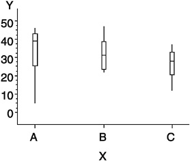
Figure 7.15: Box Plot

Note: If you use HAXIS= or VAXIS= in the PLOT statement or ORDER= in an AXIS definition to restrict the range of axis values, by default any observations that fall outside the axis range are excluded from the interpolation calculation. See the MODE= option on page 197
You cannot use the GPLOT procedure PLOT statement option AREAS= with INTERPOL=BOX.
To increase the thickness of all box plot lines, including the box, whiskers, join line, and top and bottom ticks , use the WIDTH= option.
To increase the width of the box itself, use the BWIDTH= option. By default the value of BWIDTH= is the same as the value of WIDTH=. Therefore, if you specify a value for WIDTH= and omit BWIDTH=, the width of the box changes.

For a scatter effect with the box, use a multiple plot request, as in this example:

 symbol1 i=none v=star color=green;  symbol2 i=box v=none color=blue;  proc gplot data=test;     plot (y y)*x / overlay;

This option cannot be used in a symbol definition that is named in the GPLOT procedure, when that procedure is generating output for the Web using a Java device driver. This applies only when the PLOT statement is used with the OVERLAY option, or when the PLOT2 statement is used, with or without the OVERLAY option.
Featured in: Example 4. Creating and Modifying Box Plots on page 233.
Not supported by: Java (partial)

INTERPOL=HILO<C>< option >

I=HILO<C>< option >

specifies that a solid vertical line connect the minimum and maximum Y values for each X value. The data should have at least two values of Y for every value of X; otherwise , the single value is displayed without the vertical line.
By default, for each X value, the mean Y value is marked with a tick. This is shown in Figure 7.16 on page 190.

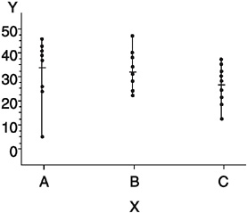
Figure 7.16: High-Low Plot

To specify high, low, close stock market data, include this option:

C	draws tick marks at the close value instead of at the mean value. Specifying C assumes that there are three values of Y (HIGH, LOW, and CLOSE) for every value of X. If more or fewer than three Y values are specified, the mean is ticked . The Y values can be in any order in the input data set.
In addition, you can specify one of these values for option :
B	connects the minimum and maximum Y values with bars instead of lines. Use the BWIDTH= option to increase the width of the bars.
J	joins the mean values or the close values (if HILOC is specified) with a line. This point is not marked with a tick mark. You cannot use the PLOT statement option AREAS= with INTERPOL=HILOJ.
T	adds tops and bottoms to each line.
BJ	connects maximum and minimum values with a bar and joins the mean or close values.
TJ	adds tops and bottoms to the lines and joins the mean or close values.

Figure 7.16 on page 190 shows the type of plot INTERPOL=HILO produces. Plot symbols in the form of dots have been added to this figure.
To increase the thickness of all lines generated by the INTERPOL=HILO option, use the WIDTH= option.
Note: If you use HAXIS= or VAXIS= in the PLOT statement or ORDER= in an AXIS definition to restrict the range of axis values, by default any observations that fall outside the axis range are excluded from the interpolation calculation. See the option MODE= on page 197.
This option cannot be used in a symbol definition that is named in the GPLOT procedure, when that procedure is generating output for the Web using a Java device driver. This applies only when the PLOT statement is used with the OVERLAY option, or when the PLOT2 statement is used, with or without the OVERLAY option.
Featured in: Example 1. Ordering Axis Tick Marks with SAS Datetime Values on page 226.
Not supported by: Java (partial)

INTERPOL=JOIN

I=JOIN

connects data points with straight lines. Points are connected in the order they occur in the input data set. Therefore, the data should be sorted by the independent (horizontal axis) variable.
If the data contain missing values, the observations are omitted. However, the plot line is not broken at missing values unless the SKIPMISS option is used.
See also: the SKIPMISS on page 1112 option and Missing Values on page 1087.

INTERPOL=L< degree ><S>

I=L< degree ><S>

specifies a Lagrange interpolation to smooth the plot line. Specify one of these values for degree :

1 3 5	specifies the degree of the Lagrange interpolation polynomial. By default, degree is 1.
In addition, you can specify one or both of these:
P	specifies a parametric interpolation
S	sorts a data set by the independent variable before plotting its data.

The Lagrange methods are useful chiefly when data consist of tabulated, precise values. A polynomial of the specified degree (1, 3, or 5) is fitted through the nearest 2, 4, or 6 points. In general, the first derivative is not continuous. If the values of the horizontal variable are not strictly increasing, the corresponding parametric method (L1P, L3P, or L5P) is used.
Specifying INTERPOL=L1P, INTERPOL=L3P, or INTERPOL=L5P results in a parametric Lagrange interpolation of degree 1, 3, or 5, respectively. Both the horizontal and vertical variables are processed with the Lagrange method and a parametric interpolation of degree 1, 3, or 5, using the distance between points as a parameter.

INTERPOL= map/plot-pattern

I= map/plot-pattern

specifies that a pattern fill the polygon that has been defined by the data points. Values for map/plot-pattern are

MEMPTY
ME
- an empty pattern. EMPTY and E are valid aliases.
- The Java applet does not support this option.
MSOLID
MS
- a solid pattern. SOLID and S are valid aliases

M density < style < angle >>

a shaded pattern. (The Java applet does not support this option.)

Density specifies the density of the pattern s shading:

1...5	1 produces the lightest shading and 5 produces the heaviest.
Style specifies the direction of pattern lines:
N	parallel lines (the default)
X	crosshatched lines.
Angle specifies the starting angle for parallel or crosshatched lines:
0...360	the degree at which the parallel lines are drawn. By default, angle is 0 (lines are parallel to the horizontal axis).

The INTERPOL= map/plot-pattern option only works if the data are structured so that the data points and, consequently, the plot lines form an enclosed area. The plot lines should not cross each other.
See also: the PATTERN Statement on page 169
Featured in: Example 5. Filling the Area between Plot Lines on page 236
Not supported by: Java (partial)

INTERPOL=NEEDLE

I=NEEDLE

draws a vertical line from each data point to a horizontal line at the 0 value on the vertical axis or the minimum value on the vertical axis if it is greater than 0. The horizontal line is drawn automatically.
Figure 7.17 on page 192 shows the type of plot INTERPOL=NEEDLE produces. Plot symbols are not displayed in this figure.

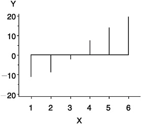
Figure 7.17: Needle Plot
You cannot use the PLOT statement option AREAS= with INTERPOL=NEEDLE.

INTERPOL=NONE

I=NONE

suppresses any interpolation and, if VALUE= is not specified, also suppresses plot points. If no interpolation method is specified in a SYMBOL statement and if the graphics option INTERPOL= is not used, INTERPOL=NONE is the default.
You cannot use the PLOT statement option AREAS= with INTERPOL=NONE.

INTERPOL=R< type ><0><CLM CLI<50...99>>

I=R< type ><0><CLM CLI<50...99>>

specifies that a plot is a regression analysis. By default, regression lines are not forced through plot origins and confidence limits are not displayed.

Type specifies the type of regression. Specify one of these values for type :

L	requests linear regression representing the regression equation Y= ² + ² ₁ X
Q	requests quadratic regression representing the regression equation Y= ² + ² ₁ X + ² ₂ X ²
C	requests cubic regression representing the regression equation Y= ² + ² ₁ X+ ² ₂ X ² + ² ₃ X ³
	Note: When least-square solutions for the parameters are not unique, the SAS/GRAPH server defaults to a quadratic equation for the interpolation whereas the Java client and ActiveX client might pick a cubic solution to use.
By default, type is L. The regression line is drawn in the line type specified in the LINE= option. By default, the type of the regression line is 1.
Note: You must specify type if you use either 0, or CLI, or CLM. To force the regression line through a (0,0) origin, specify:
	eliminates the ² parameter, or intercept, from the regression equation. If the origin is at (0,0), also forces the regression line through the origin. For example, if you specify 0 for a linear regression, the plot line represents the equation Y= ² ₁ X
	Note: To force the regression line through the origin (0,0) when the data ranges do not place the origin at (0,0), use the GPLOT procedure options HZERO and VZERO (ignored if the data contain negative values), or use HAXIS and VAXIS to specify axes ranges from 0 to maximum data value. If the data ranges contain negative values and HAXIS and VAXIS specify ranges starting at 0, only values within the displayed range are used in the interpolation calculations.
To display confidence limits, specify one of these:
CLM	displays confidence limits for mean predicted values
CLI	displays confidence limits for individual predicted values.
You can specify confidence levels from 50% to 99%. By default, the confidence level is 95%. Include a confidence level specification only if you use CLM or CLI.
The line type used for the confidence limit lines is determined by adding 1 to the values of LINE=. By default, the line type of confidence limit lines is 2.
Figure 7.18 on page 193 shows the type of plot INTERPOL=RCCLM95 produces (cubic regression analysis with 95% confidence limits).

click to expand
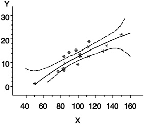
Figure 7.18: Plot of Regression Analysis and Confidence Limits

Featured in: Example 4 on page 1126.
Not supported by: Java (partial)

INTERPOL=SM< nn ><S>

I=SM< nn ><S>

specifies that a smooth line is fit to data using a spline routine. INTERPOL=SM is a method for smoothing noisy data. The points on the plot do not necessarily fall on the line.

The relative importance of plot values versus smoothness is controlled by nn . Values for nn are

0...99	produces a cubic spline that minimizes a linear combination of the sum of squares of the residuals of fit and the integral of the square of the second derivative (Reinsch 1967) ^[*] . The greater the nn value, the smoother the fitted curve. By default, the value of nn is 0.
In addition, specify one or both of these:
P	specifies a parametric cubic spline
S	sorts data by the independent variable before plotting.
Not supported by: Java
^[] Reinsch, C.H. (1967), Smoothingby Spline Functions, Numerische Mathematik* , 10, 177 “183.

INTERPOL=SPLINE<S>

I=SPLINE<S>

specifies that the interpolation for the plot line use a spline routine. INTERPOL=SPLINE produces the smoothest line and is the most efficient of the nontrivial spline interpolation methods.
Spline interpolation smoothes a plot line using a cubic spline method with continuous second derivatives (Pizer 1975) ^[**] This method uses a piecewise third-degree polynomial for each set of two adjacent points. The polynomial passes through the plotted points and matches the first and second derivatives of neighboring segments at the points.

Specify one or both of these:

P	specifies a parametric spline interpolation method. This interpolation uses a parametric spline method with continuous second derivatives. Using the method described earlier for the spline interpolation, a parametric spline is fitted to both the horizontal and vertical values. The parameter used is the distance between points

	If two points are so close together that the computations overflow, the second point is not used.
S	sorts a data set by the independent variable before plotting its data.

Note: When points on the graph are out of range of the axis values, the curve is clipped. If an end point is out of range, no curve is drawn. Out-of-range conditions may be caused by restricting the range of axis values with the HAXIS= or VAXIS= option in the PLOT statement or the ORDER= option in an AXIS definition.
Note: When points on the graph are close together and a spline interpolation is used, the Java applet is unable to draw some line types correctly.

INTERPOL=STD<1 2 3>< variance >< option(s) >

I=STD<1 2 3>< variance >< option(s) >

specifies that a solid line connect the mean Y value with ± 1, 2, or 3 standard deviations for each X.

Note: By default, 2 standard deviations are used.

The sample variance is computed about each mean, and from it, the standard deviation s _y is computed. Variance can be one or both of these:

M	computes ,
P	computes sample variances using a pooled estimate, as in a one-way ANOVA model.
In addition, specify one of these values for option(s) :
B	connects the minimum and maximum Y values with bars instead of lines.
J	connects the means from bar to bar with a line.
T	adds tops and bottoms to each line.
BJ	connects maximum and minimum values with a bar and joins the mean values.
TJ	adds tops and bottoms to the lines and joins the mean values.
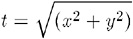
Figure 7.19 on page 195 shows the type of plot INTERPOL=STD produces. A horizontal tick is drawn at the mean. Plot symbols in the form of dots have been added to this figure.

click to expand
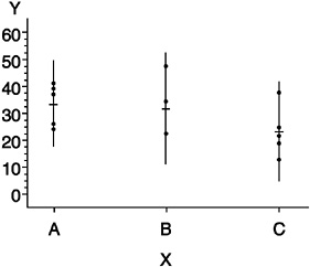
Figure 7.19: Plot of Standard Deviations

Note: By default, the vertical axis ranges from the minimum to the maximum Y value in the data. If the requested number of standard deviations from the mean covers a range of values that exceeds the maximum or is less than the minimum, the STD lines are cut off at the minimum and maximum Y values. When this cutoff occurs, rescale the axis using VAXIS= in the PLOT statement or ORDER= in an AXIS definition so that the STD lines are shown.
If you restrict the range of axis values by using HAXIS= or VAXIS= in a PLOT statement or ORDER= in an AXIS definition, by default any observations that fall outside the axis range are excluded from the interpolation calculation. See the MODE= on page 197 option.
To increase the thickness of all lines generated by the INTERPOL=STD option, use the WIDTH= option.
You cannot use the PLOT statement option AREAS= with INTERPOL=STD.
This option cannot be used in a symbol definition that is named in the GPLOT procedure, when that procedure is generating output for the Web using a Java device driver. This applies only when the PLOT statement is used with the OVERLAY option, or when the PLOT2 statement is used, with or without the OVERLAY option.
Not supported by: Java (partial)

INTERPOL=STEP< placement ><J><S>

I=STEP< placement ><J><S>

specifies that the data are plotted with a step function. By default, the data point is on the left of the step, the steps are not joined with a vertical line, and the data are not sorted before processing.

Specify one of these values for placement :

L	displays the data point on the left of the step.
R	displays the data point on the right of the step.
C	displays the data point in the center of the step.
	Note: When a step is retraced in order to locate its center point, both the server and Java treat this as effectively not drawing that part of the step at all. ActiveX, however, draws each part of the step ”resulting in a somewhat differently appearing graph.
In addition, specify one or both of these:
J	produces steps joined with a vertical line.
S	sorts unordered data by the independent variable before plotting.
Figure 7.20 on page 196 shows the type of plot INTERPOL=STEPJR produces. Plot symbols in the form of dots have been added to this figure.

click to expand
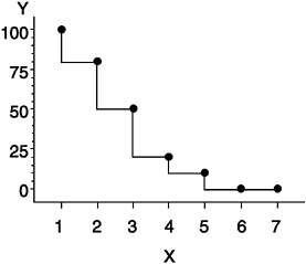
Figure 7.20: Step Plot

LINE= line-type

L= line-type

specifies the line type of the plot line in the GPLOT procedure, or the contour line in the GCONTOUR procedure:

1

a solid line.

2...46

a dashed line.

Line types are shown in Figure 7.22 on page 208. By default, LINE=1.
Note: This option overrides the LineStyle attribute in graph styles. For more information on graph styles, see SAS Output Delivery System: User s Guide .
Neither the Java applet nor ActiveX control supports client-side rendering for GCONTOUR.
Not supported by: Java (partial), ActiveX (partial)

MODE=EXCLUDE INCLUDE

specifies that interpolation calculations exclude or include data values that are outside the range of plot axes. By default, MODE=EXCLUDE, which excludes values outside the axis range from any calculations.
If you control the range of values displayed on an axis by using HAXIS= and VAXIS= in the GPLOT procedure, or ORDER= in an AXIS definition, any data points that lie outside of the range of the axes are discarded before the calculations are done for interpolation lines. This has a particularly noticeable effect on the high-low interpolation methods, which include INTERPOL=HILO, INTERPOL=BOX, and INTERPOL=STD. Regression analysis also represents only part of the original data.
See also: Values Out of Range on page 1087.

POINTLABEL<=( label-description(s) ) NONE>

labels plot points. The labels always use the format that is assigned to the variable(s) whose values are used for the labels. POINTLABEL without any specified descriptions labels points with the Y value. NONE suppresses the point labels. Label-description(s) can be used to change the variable whose values are used to label points, and/or to change features of the label text, such as the color, font, or size of the text.
Note: If you do not specify a color on a SYMBOL statement, the symbol definition is rotated through the colors list before the next SYMBOL statement is used. Thus, if your plot contains multiple plot lines and you want to limit your POINTLABEL specification to a single line, you must specify a color on the SYMBOL statement that contains the POINTLABEL description.
Label-description(s) can be one or more of these:
- COLOR= text-color
- C= text-color
 - specifies the color of the label text. The default is the first color from the colors list.
- FONT= font NONE
- F= font NONE
 - specifies the font for the text. See Chapter 5, SAS/GRAPH Fonts, on page 75 for details on specifying font . If you omit FONT=, a font specification is searched for in this order:
 1. the FTEXT= option in a GOPTIONS statement
 2. the default hardware font, NONE.
- HEIGHT= text-height < units >
- H= text-height < units >
 - specifies the height of the text characters in number of units. By default, HEIGHT=1 CELL . If you omit HEIGHT=, a text height specification is searched for in this order:
 1. the HTEXT= option in a GOPTIONS statement
 2. the default value, 1.
- JUSTIFY=CENTER LEFT RIGHT
- J=C L R
 - specifies the horizontal alignment of the label text. The default is CENTER. The location of the point label is relative to the location of the corresponding data point.

POSITION=TOP MIDDLE BOTTOM
- specifies the vertical placement of the label text. The default is TOP. The location of the point label is relative to the location of the corresponding data point.

# var # x :# y <$ char > # y :# x <$ char >
- specifies the variable(s) whose values will label the plot points. The variable specification must be enclosed in either single or double quotation marks. The first specified variable must be prefixed with a pound sign (#). If a second variable is specified, it must be prefixed with a colon and a pound sign (:#). Optionally, when you specify both the X and Y variables, you can specify the character to display as the delimiter between variable values in the plot label.
- By default if POINTLABEL is specified without naming a label variable, the Y values label the plot points. You can change the default by using #var to specify a different variable whose values should label the points. For example, you might specify the name of the X variable. The following option specifies the variable SALES as the variable whose values will label plot points:
```
 POINTLABEL=("#sales") 
```
- Alternatively, you can label the plot points with the values of the X and Y variables, in either order. The order that you specify X and Y in the variable specification determines the order that the values are displayed in the label. The following option specifies variables HEIGHT and WEIGHT; in the label, the value for HEIGHT will be displayed, followed by the value for WEIGHT:
```
 POINTLABEL=("#height:#weight") 
```
- The variables that you specify must be the plot s X and Y variables. Specifying any other variables will cause unexpected labeling.
- By default when you specify both the X and Y variables, a colon (:) displays in the label to separate the values in each label. To change the character that displays as the delimiter, use the $ syntax to specify an alternative character. The following option specifies a vertical bar () as the delimiter in the label:
```
 POINTLABEL=("#height:#weight $") 
```
- The $ syntax must be within the same quotation marks as the variable specification. The $ specification can precede or follow the variable specification, but it must be separated from the variable specification by at least one space.
- Note: Specifying a delimiting character with the $ only changes the character that displays in the label. It does not change the syntax of the variable specification, which requires a colon and pound sign (:#) to precede the second variable.
- Note: There is a sixteen character length limit for each variable. A maximum character length limit of thirty-three characters is possible. This can be composed of X and Y variables, any other valid data set variable, and a separator as required.
Specify as many label-description suboptions as you want. Enclose them all within a single set of parentheses, and separate each suboption from the others by at least one space.
Not supported by: Java (partial), ActiveX (partial)

REPEAT= number-of-times

R= number-of-times

specifies the number of times that a SYMBOL definition is applied before the next SYMBOL definition is used. By default, REPEAT=1.
The behavior of REPEAT= depends on whether any of the SYMBOL color options (CI=, CV=, CO=, and COLOR=) or the CSYMBOL= graphics option also is used:
- If any SYMBOL color option also is used in the SYMBOL definition, that SYMBOL definition is repeated the specified number of times in the specified color.
- If no SYMBOL color option is used but the CSYMBOL= graphics option is currently in effect, the SYMBOL definition is repeated the specified number of times in the specified color.
- If no SYMBOL statement color options are used and the CSYMBOL= graphics option is not used, the SYMBOL definition is cycled through each color in the colors list, and then the entire group generated by this cycle repeats the number of times specified by REPEAT=. Thus, the total number of iterations of the SYMBOL definition depends on the number of colors in the current colors list.
  
  Neither the Java applet nor ActiveX control supports client-side rendering for GCONTOUR.
See also: Using the SYMBOL Statement on page 202.
Not supported by: Java (partial), ActiveX (partial)

SINGULAR= n

tunes the algorithm used to check for singularities. The default value is machine dependent but is approximately 1E-7 on most machines. This option is rarely needed.

STEP= distance < units >

specifies the minimum distance between labels on contour lines. The value of distance must be greater than zero. By default, STEP=65PCT.
Note: If you specify units of PCT or CELLS, STEP= calculates the distance between the labels based on the width of the graphics output area, not the height. For example, if you specify STEP=50PCT and if the graphics output area is 9 inches wide, the distance specified is 4.5 inches. A value less than 10 percent is ignored and 10 percent is used instead.
When you use STEP=, specify the minimum distance that you want between labels. The option then calculates how many labels it can fit on the contour line, taking into account the length of the labels and the minimum distance you specified. Once it has calculated how many labels it can fit while retaining the minimum distance between them, it places the labels, evenly spaced , along the line. Consequently, the space between labels may be greater than what you specify, although it will never be less.
In general, to increase the number of labels from the default, reduce the value of distance .
If the procedure cannot write the label at a particular location on the contour, for example because the contour line makes a sharp turn , the label may be placed farther along the line or omitted. If labels are omitted, a note appears in the log. Specifying a low value for the GCONTOUR procedure s TOLANGLE= option may also cause labels to be omitted, since this forces the procedure to select smoother labeling locations, which may not be available on some contours .
Featured in: Example 2 on page 906.
Not supported by: Java, ActiveX

VALUE= special-symbol text-string NONE

V= special-symbol text-string NONE

- specifies a plot symbol for the data points (GPLOT and GBARLINE). If you omit the SYMBOL statement, plot points are generated using the default plot symbol. The default symbol is a square if you use the ActiveX or Java devices and a PLUS sign for other devices. If you specify a SYMBOL statement, but do not specify the VALUE= option, plot symbols are suppressed.
  
  Note: For ActiveX output, the VALUE= option is not supported when INTERPOL=HILO or INTERPOL=STD. You can use the OVERLAY option with GPLOT to get symbols to appear on the data points.
- specifies contour-label text in a contour plot (GCONTOUR). By default with the AUTOLABEL option, GCONTOUR labels contour lines with the contour variable s value at that contour level.
- VALUE=NONE suppresses plot symbols at the data points, or labels on the contour lines. You can set the VALUE=NONE option independent of the INTERPOL= option.
Values for special-symbol are the names and characters shown in Figure 7.21 on page 202. The special symbol table can be used only if the FONT= option is not used or a null value is specified:
```
 font=, 
```
Note: To specify a single quotation mark, you must enclose it in double quotation marks:
```
 value="" 
```
To specify a double quotation mark, you must enclose it in single quotation marks:
```
 value=" 
```
In some operating environments, punctuation characters may require single quotes.
If you use VALUE= text-string to specify a plot symbol, you must also use the FONT= option to specify a symbol font or a text font. If you specify a symbol font, the characters in the string are character codes for the symbols in the font. If you specify a text font, the characters in the string are displayed. If you specify a text string containing quotes or blanks, enclose the string in single quotes.
For example, if you specify this statement, the plot symbol is the word "plus" instead of the symbol +:
```
 symbol font=swiss value=plus; 
```

Java and ActiveX support the following characters from the marker font for special-symbol :

Character	Aliases
Marker	Cone, Pyramid, Default
Square	Cube
Star
Circle	Sphere, Dot, Balloon
Plus	Cross
Flag	Y
X
Prism	Z
Spade
Heart	#
Diamond	$
Club	%
Hexagon	Paw
Cylinder	Hash

Note: If you do not use a SYMBOL statement to specify a color for each symbol, but you do specify a colors list in a GOPTIONS statement, then Java and ActiveX assign colors to symbols differently than does the SAS server. To ensure consistency on all devices, you should specify the desired color of each symbol.The SAS server restarts at the first color in the colors list and rotates through all of the colors in the color list for the first default symbol before going to the next symbol in the default symbol list where it again rotates through all of the colors in the color list before picking up the next symbol.
Note: The VALUE option overrides the MarkerSymbol attribute in graph styles. For more information on graph styles, see SAS Output Delivery System: User s Guide .
See also: the option FONT= on page 186 and Specifying Plot Symbols on page 205.
Featured in: Example 3. Rotating Plot Symbols through the Colors List on page 231, Example 4. Creating and Modifying Box Plots on page 233, and Example 2 on page 906.
Not supported by: Java (partial), ActiveX (partial)

WIDTH= thickness-factor

W= thickness-factor

specifies the thickness of interpolated lines (GPLOT) or contour lines (GCONTOUR), where thickness-factor is a number. The thickness of the line increases directly with thickness-factor . By default, WIDTH=1.
WIDTH= also affects all the lines in box plots (INTERPOL=BOX), high-low plots with bars (INTERPOL=HILOB), and standard deviation plots (INTERPOL=STD). It also affects the outlines of the area generated by the AREAS= option in the PLOT statement of the GPLOT procedure.
Note: By default, the value specified by WIDTH= is used as the default value for the BWIDTH= option. For example, specifying WIDTH=6 also sets BWIDTH= to 6 unless you explicitly assign a value to BWIDTH=.
Java and ActiveX do not provide the same measure of control for width as SAS/ GRAPH on the server. Measurements are translated to pixels rather than a percentage.
Featured in: Example 1. Ordering Axis Tick Marks with SAS Datetime Values on page 226 and Example 4. Creating and Modifying Box Plots on page 233.
Not supported by: Java (partial) and ActiveX (partial)
Note: The words or special characters in the VALUE= column are entered exactly as shown.

Using the SYMBOL Statement

A SYMBOL statement specifies one or more options that indicate the color and other attributes used by the GPLOT procedure or the GCONTOUR procedure. For GPLOT, the main attributes include the plot symbol, interpolation method, and type of plot line. For GCONTOUR, the main attributes include the type of contour lines used and the text used to label those lines.

Note: SYMBOL statements can only be applied to contour plots when the AUTOLABEL option is specified on GCONTOUR.

You can define up to 99 different SYMBOL statements. A SYMBOL statement without a number is treated as a SYMBOL1 statement.

SYMBOL definitions can be defined anywhere in your SAS program. They are global and remain in effect until canceled or until you end your SAS session. Once defined, SYMBOL definitions can be

assigned by default by GPLOT or explicitly selected with the plot request
used by GCONTOUR to control the labels and attributes of contour lines.

SYMBOL statements generate one or more symbol definitions, depending on how color is used and whether a plot symbol or type of contour line is specified. For more information, see Controlling Consecutive SYMBOL Statements on page 203 and Using Generated Symbol Sequences on page 208.

Although it is common practice, you do not have to start with SYMBOL1, and you do not have to use sequential statement numbers . When assigning SYMBOL definitions, SAS/GRAPH software starts with the lowest -numbered definition and works upward, ignoring gaps in the numbering.

Altering or Canceling SYMBOL Statements

SYMBOL statements are additive. If you define a SYMBOL statement and later submit another SYMBOL statement with the same number, the new SYMBOL statement defines or cancels only the options that are included in the new statement. Options that are not included in the new statement are not changed and remain in effect.

Assume you define SYMBOL4 as:

 symbol4 value=star cv=red height=4;

The following statement cancels only HEIGHT= without affecting the rest of the definition:

 symbol4 height=;

Add or change options in the same way. This statement adds an interpolation method to SYMBOL4:

 symbol4 interpol=join;

This statement changes the color of the plot symbol from red to blue:

 symbol4 cv=blue;

After all these modifications, SYMBOL4 has these characteristics:

 symbol4 value=star cv=blue interpol=join;

Cancel individual SYMBOL statements by defining a SYMBOL statement of the same number without options (a null statement):

 symbol4;

Canceling one SYMBOL statement does not affect any other SYMBOL definitions. To cancel all current SYMBOL statements, use RESET= in a GOPTIONS statement:

 goptions reset=symbol;

Specifying RESET=GLOBAL or RESET=ALL cancels all current SYMBOL definitions as well as other settings.

To display current SYMBOL definitions in the LOG window, use the GOPTIONS procedure with the SYMBOL option:

 proc goptions symbol nolist;  run;

Controlling Consecutive SYMBOL Statements

If you specify consecutively numbered SYMBOL statements and you want SAS/GRAPH to use each definition only once, use color specifications to ensure each SYMBOL statement generates only one symbol definition. You can

specify colors on each SYMBOL statement, using the COLOR=, CI=, CV=, or CO= options. This method lets you explicitly assign colors for each definition. For example, these statements generate two definitions:
```
 symbol1 value=star color=green;  symbol2 value=square color=yellow; 
```
specify a default color for all SYMBOL statements using the CSYMBOL= option on the GOPTIONS statement. This method makes it easy to specify the same color for each definition when you do not need more explicit color specifications.
limit the colors list to a single color using the COLORS= option on the GOPTIONS statement. This method makes it easy to specify the same color for each definition when you want the color to apply to other definitions also, such as PATTERN definitions.

For more information on specifying colors for symbol definitions, see Using Color on page 206.

If you do not use color to limit a SYMBOL statement to a single symbol definition, SAS/GRAPH generates multiple symbol definitions from that statement by rotating the current definition through the colors list (for more details, see Using Generated Symbol Sequences on page 208). Because SAS/GRAPH uses symbol definitions in the order they are generated, this means that the n th symbol definition applied to a graph does not necessarily correspond to the SYMBOL n statement.

For example, assuming no color is specified on the CSYMBOL= graphics option, these statements generate four definitions:

 goptions colors=(red blue green);  symbol1 value=star;  symbol2 value=square color=yellow;

Because no color is specified on SYMBOL1, SAS/GRAPH rotates the symbol definition through the colors list, which has three colors. Thus, SYMBOL1 defines the first three applied symbol definitions, and SYMBOL2 defines the 4th:

Sequence Number	Source	Characteristics: Color	Symbol
1	SYMBOL1	red	star
2	SYMBOL1	blue	star
3	SYMBOL1	green	star
4	SYMBOL2	yellow	square

In this case, if a graph needs only three symbols, the SYMBOL2 definition is not used.

To make the n th applied symbol definition correspond to the SYMBOL n statement, limit each SYMBOL statement to a single color, using one of the techniques listed at the beginning of this section.

Setting Definitions for PROC GPLOT

The following topics apply only for SYMBOL statements used with PROC GPLOT:

specifying plot symbols
specifying default interpolation methods
sorting data with spline interpolation.

Specifying Plot Symbols

The VALUE= option specifies the plot symbols that PROC GPLOT uses to mark the data points on a plot. Plot symbols can be

special symbols from Figure 7.21 on page 202
characters from symbol fonts
text strings.

By default, the plot symbol is the + symbol. To specify a special symbol, use VALUE= to specify a name or a character from Figure 7.21 on page 202:

 symbol1 value=hash color=green;  symbol2 value=) color=blue;

This example uses color to ensure each SYMBOL statement generates only one definition. You can omit color specifications to let SAS/GRAPH rotate symbol definitions through the colors list. For details, see Using Generated Symbol Sequences on page 208.

To use plot symbols other than those in Figure 7.21 on page 202, use the FONT= option to specify a font for the plot symbol. If the font is a symbol font, such as Marker, the string specified with the VALUE= option is the character code for the symbol to be displayed. If the font is a text font, the string specified with VALUE= is displayed as the plot symbol. (See VALUE= on page 199 and FONT= on page 186.)

This table illustrates some of the ways you can define a plot symbol:

Definition	Plot Symbol
symbol1 value=plus;
symbol2 value=+;
symbol3 font=swiss value=plus;	plus
symbol4 font=marker value=U;	–
symbol5value=" ";

Specifying a Default Interpolation Method

The INTERPOL= option in a GOPTIONS statement specifies a default interpolation method to be used with all SYMBOL definitions. This default interpolation method is in effect unless you specify a different interpolation in a SYMBOL statement. If the GOPTIONS statement does not specify an interpolation method, the default for each SYMBOL statement is NONE.

Sorting Data with Spline Interpolation

If you want the GPLOT procedure to sort by the horizontal axis variable before plotting, add the letter S to the end of any of the spline interpolation methods (INTERPOL=L, INTERPOL=SM, and INTERPOL=SPLINE). For example, suppose you want to overlay three plots (Y1*X1, Y2*X2, and Y3*X3) and for each plot, you want the X variable sorted in ascending order. Use these statements:

 symbol1 i=splines c=red;  symbol2 i=splines c=blue;  symbol3 i=splines c=green;  proc gplot;     plot y1*x1 y2*x2 y3*x3 / overlay;  run;

Using Color

Generally, there are two ways to explicitly specify color for SYMBOL statements:

specify colors on the SYMBOL statements
specify a color on the CSYMBOL= graphics option.

You can also let SAS/GRAPH rotate symbol definitions through the colors list. For details, see Using Generated Symbol Sequences on page 208.

Specifying Colors with SYMBOL Statements

The SYMBOL statement has these options for specifying color:

The CV= option specifies color for plot symbols in GPLOT, or for contour labels in GCONTOUR.
The CO= option specifies color for confidence limit lines and area outlines in GPLOT.
The CI= option specifies color for plot lines in GPLOT, or contour lines in GCONTOUR.
The COLOR= option specifies color for the entire symbol. For GPLOT, this includes plot symbols, plot lines, and outlines. For GCONTOUR, this includes contour lines and labels.

CV= and CI= have the same effect as using COLOR= when they are used in these ways:

Only CV= or CI= option is used. (The option that is not used is assigned the value of the option used.)
Both CV= and CI= specify the same color.

In general, CI=, CV=, and CO= color specific areas of the symbol. Use these options to produce symbols and plot lines of different colors without having to overlay multiple plot pairs. For example, if you request regression analysis with confidence limits, use this statement to assign red to the plot symbol, blue to the regression lines, and green to the confidence limit lines:

 symbol cv=red ci=blue co=green;

The COLOR= option colors the entire symbol or those portions of it not colored by one of the other color options. If COLOR= precedes CI= or CV=, the CI= or CV= specification is used instead. If none of the SYMBOL color options is used, color specifications are searched for in this order:

the CSYMBOL= option in a GOPTIONS statement
each color in the colors list sequentially before the next SYMBOL definition is used.

CAUTION:

If no color options are used, the SYMBOL definition cycles through each color in the colors list.

If the SYMBOL color options and the CSYMBOL= graphics option are not used, the SYMBOL definition cycles through each color in the colors list before the next definition is used. For details, see Using Generated Symbol Sequences on page 208.

Specifying Color with CSYMBOL=

The CSYMBOL= option on the GOPTIONS statement specifies the default color to be used by all SYMBOL definitions:

 goptions csymbol=green;  symbol1 value=star;  symbol2 value=square;

In this example, both SYMBOL statements use green.

CSYMBOL= is overridden by any of the SYMBOL statement color options. See Using Color on page 206 for details.

If more SYMBOL definitions are needed, SAS/GRAPH returns to generating default symbol sequences.

Specifying Line Types

To specify the type of line for plot or contour lines, use the LINE= option to specify a number from 1 through 46. Figure 7.22 on page 208 shows the line types represented by these numbers. By default, the line type is 1 for plot and contour lines, and 2 for confidence limit lines.

Note: These line types are also used by other statements and procedures. Some options accept a line type of 0, which produces no line.

Using Generated Symbol Sequences

Symbol sequences are sets of SYMBOL definitions that are automatically generated by SAS/GRAPH software if any of these conditions is true:

no valid SYMBOL definition is available. In this case, default symbol sequences are generated by rotating symbol definitions through the color specified on the GOPTIONS statement s CSYMBOL= option. If a CSYMBOL= color is not in effect, the definitions are rotated through the colors list.
a SYMBOL statement specifies color but not a plot symbol for the GPLOT procedure, or a line type for the GCONTOUR procedure (assuming GCONTOUR does not specify the needed line types). In this case, a default plot symbol or line type is used with the specified color and only one definition is generated.
a SYMBOL statement specifies a plot symbol for GPLOT or a line type for GCONTOUR, but no color options. In this case, the specified plot symbol or line type is used once with the color specified by the CSYMBOL= graphics option. If a CSYMBOL= color is not in effect, the specified plot symbol or line type is rotated through the colors list.

If REPEAT= is also used, the resulting SYMBOL definition is repeated the specified number of times.

Default Symbol Sequences

Default symbol sequences are generated by rotating symbol definitions through the current colors list.

Definitions used for GPLOT rotate plot symbols through the colors list; the first default plot symbol is a plus sign (+).
Definitions used for GCONTOUR rotate line types; the first default line type is a solid line (line type 1).

Each time a default definition is required, SAS/GRAPH takes the first default plot symbol or line type and uses it with the first color in the colors list. If more than one definition is required, it uses the same plot symbol or line type with the next color in the colors list and continues until all the colors have been used once. If more definitions are needed, SAS/GRAPH selects the second default plot symbol or line type and rotates it through the colors list. It continues in this fashion, selecting default plot symbols or line types and cycling them through the colors list until all the required definitions are generated.

If a color has been specified with the CSYMBOL= option on the GOPTIONS statement, each default plot symbol or line type is used once with the specified color, and the colors in the colors list are ignored.

Symbol Sequences Generated from SYMBOL Statements

If a SYMBOL statement does not specify color, and if the CSYMBOL= graphics option is not used, the symbol definition is rotated through every color in the colors list before the next SYMBOL definition is used:

 goptions colors=(blue red green);  symbol1 cv=red i=join;  symbol2 i=spline v=dot;  symbol3 cv=green v=star;

Here, the SYMBOL1 statement generates the first SYMBOL definition. The SYMBOL2 statement does not include color, so the first default plot symbol is rotated through all colors in the colors list before the SYMBOL3 statement is used. This table shows the colors and symbols that would be used if nine symbol definitions were required for PROC GPLOT:

Sequence Number		Characteristics:
Sequence Number	Source	Color	Symbol	Interpolation
1	SYMBOL1	cv=red	first default	join
2	SYMBOL2	color=blue	dot	spline
3	SYMBOL2	color=red	dot	spline
4	SYMBOL2	color=green	dot	spline
5	SYMBOL3	cv=green	star	NONE
6	first default	color=blue	first default	default
7	first default	color=red	first default	default
8	first default	color=green	first default	default
9	second default	color=blue	second default	default

Notice that after the SYMBOL statements are exhausted, the procedure begins using the default definitions (sequences 6 through 9). Each plot symbol from the default list is rotated through all colors in the colors list before the next plot symbol is used. Also, SYMBOL1 does not specify a plot symbol, so the default sequencing provides the first default symbol (a + sign). When sequencing resumes in sequence number 6, it starts at the beginning again, selecting the first default plot symbol and rotating it through the colors list.

If you use REPEAT= but no color, the sequence generated by cycling the definition through the colors list is repeated the number of times specified by REPEAT=. For example, these statements define a colors list and illustrate the effect of REPEAT= on SYMBOL statements both with and without explicit color specifications:

 goptions colors=(blue red green);  symbol1 color=gold repeat=2;  symbol2 value=star color=cyan;  symbol3 value=square repeat=2;

Here, SYMBOL1 is used twice, SYMBOL2 is used once, and SYMBOL3 rotates through the list of three colors and then repeats this cycle a second time:

Sequence Number		Characteristics:
Sequence Number	Source	Color	Symbol	Interpolation
1	SYMBOL1	gold	first default	default
2	SYMBOL1	gold	first default	default
3	SYMBOL2	cyan	star	default
4	SYMBOL3	blue	square	default
5	SYMBOL3	red	square	default
6	SYMBOL3	green	square	default
7	SYMBOL3	blue	square	default
8	SYMBOL3	red	square	default
9	SYMBOL3	green	square	default

^[**] Pizer, Stephen M. (1975), Numerical Computing and Mathematical Analysis , Chicago: Science Research Associates, Inc., Chapter 4.

1	a solid line.
2...46	a dashed line.
Line types are shown in Figure 7.22 on page 208. By default, LINE=1.