Grass

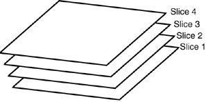
We have seen how tree rendering is a matter of providing lots of detail to a single object using very little geometry. Grass rendering is a completely different story. Each blade of grass is relatively simple and can range from a single line to a few triangles. However, we must render thousands of them to convey the look of a real grass meadow. Here complexity does not lie in the specific object but in the numbers we will try to achieve. Unsurprisingly, grass rendering methods are quite different from tree algorithms.

We will explore a series of suitable algorithms for grass. Some of them will have specific limitations (not being able to animate the grass is a popular one). Only by knowing all of the algorithms in detail will you be able to select the one that suits you best.

Layered Grass

One approach to rendering grass is to compute grass via volume rendering. This is a very low-cost algorithm that produces quite good results. The idea is simple: Take an individual blade of grass. The blade will be vertical or almost vertical, and thus simplifying it with a straight vertical line is quite accurate. But how many blades of grass exist in an open meadow? The number can be in the hundreds of thousands, and we are clearly not going to paint that many lines. The cost would be prohibitive. We need an alternative way to tackle the problem, so we can keep the apparent complexity level while keeping an actual complexity level that's low enough.

Here is where the volume rendering concept kicks in. Instead of painting individual blades, we will sample the volume occupied by the whole grass meadow, and render blades as pixels on a texture. To do so, we will use volume elements (voxels), which will encode the grass blade layout as a volume function. Now, because we are simplifying grass by straight vertical lines, we lose the Y information, and we can compress our 3D voxel to just a 2D bitmap, which we will layer in Y to convey volume.

So, our algorithm is as easy as painting the same bitmap in several Y slices. Now, the bitmap is the complex part. For volume rendering, the bitmap will need to encode the XZ section of the blades of grass. This means an RGBA bitmap, where areas covered by grass are painted with alpha=1, and areas that are not supposed to have grass blades are painted with alpha=0. It is very important to space all grass elements evenly, so we cannot sense the tiling pattern in the grass.

The rendering is quite simple. Render the ground plane first. Then, render the same quad, shifting it along Y for each iteration. Between 5 and 20 quads will be needed to convey the sense of vertical continuity. As a rule of thumb, the number of layers should be correlated to the camera's pitch. A highly pitched camera sees the blades from above, and thus not many iterations are required. A camera that is almost parallel to the ground, on the other hand, will need a much higher number of iterations to generate the illusion of a continuous blade. Take a look at Figure 20.6 for an explanatory drawing.

Figure 20.6. Layers of texture maps are used to render grass and convey parallax.

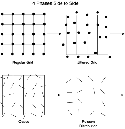
Thus, the method takes one texture map and as many quads as needed to depict the blades. We can even add animation by changing the grass texture coordinates slightly. In fact, this method has been recently coded for a variety of games and platforms. Grass cannot be looked at closely, but the illusion is quite convincing, and the cost is definitely a plus.

Additionally, this method can be implemented in a single quad using a pixel shader. Here we would compute the angles from the player to each texel and sample the volume to generate the texture map. This way we would only be using one quad, which would work the projection details internally. Notice, however, that this shader approach is not necessarily a good idea. If we paint several quads using our first approach, we can have elements half immersed in the grass realistically, such as an animal in the middle of high grass or a football standing in the middle of a field. The shader method, by using just one quad to condense the information from the different quads, eliminates this possibility.

Statistical Distribution Algorithms

We will now explore the statistical distribution algorithm, which tries to convey the density of full grass meadows in real time. Because rendering all the grass is simply impossible, the method focuses on a radius surrounding the player and alpha-fades grass as distance increases so no pop in occurs. If the grass color blends well with the terrain, the eye is fooled, and the viewer assumes that the entire meadow is effectively covered by grass. Using this simple trick ensures that we are painting a constant number of triangles for the grass, which is key to any algorithm.

Geometry is painted using quadrilateral primitives; and each quad represents several blades of grass that are grouped together. This helps reduce the triangle impact, because grass will certainly need lots of geometry. With this technique, it is important to use a good rendering method (such as Vertex Array Range [VAR] in OpenGL or DrawPrimitive in DirectX). Unfortunately, grass is not composed of primitive strips, and indexing it will not help significantly, so a VAR of quads looks like a good choice.

At this point, the statistical part of the algorithm begins its work to ensure that undesired visible patterns are broken down as much as possible. The viewer must not notice how blades are grouped together, nor notice that the landscape is not full of grass. To achieve this, the best choice is to use a spatial Poisson distribution, which distributes a series of samples in the ground plane so that the XZ distance between any two randomly selected samples is never smaller than a given threshold. Poisson distributions are popular in computer graphics literature. They are used to sample areas in stochastic ray tracing for a similar effect.

Implementing a Poisson distribution is not simple. If we need a 100 percent accurate result, the method that will need to be used is called "dart throwing;" that is, successively adding elements to the spatial distribution randomly, and if the new element violates the Poisson distribution definition (and thus has another primitive closer than the desired threshold), eliminate it. By repeating this routine until the desired density is reached, we will obtain a perfect Poisson distribution. But for large surfaces this process can take ages to complete, so a near-Poisson method is used: Divide the surface in a square grid, place one element in each node, and apply a small random movement to it in both X and Z directions. This small movement is called jitter and ensures that no visible patterns occur. If the jitter is limited (for example, to half the grid size), we still comply with a Poisson distribution at a fraction of the cost. For grass creation, this method (see Figure 20.7) will be used.

Figure 20.7. Statistical distribution of grass blades. Top left: Grid. Top right: Grid jittered to create a Poisson distribution. Bottom left: Quads added. Bottom right: Final result where all regular patterns have been eliminated.

Once the Poisson distribution has been evaluated, a rotation jitter must be introduced. Keeping all of the blade segments aligned certainly does not help convey a sense of chaos and naturalness. Thus, each quadrilateral will be rotated around the Y (vertical) axis. Here a plain random rotation will do the work perfectly, allowing a chaotic meadow to emerge.

A final step that further helps reduce visual artifacts is adding a scaling factor to the individual quads, so some quads are taller than others. A 30 percent deviation or so works well.

A note on rendering: As you have probably discovered, this is a fill-rate intensive method because many quads are required to convey the density of a real grassland. Thus, the rendering algorithm must be chosen carefully. Under OpenGL, using Display Lists is not a good idea because we will need to animate the blades and that requires resubmitting the list. A better move is to use server-side vertex arrays, which can be updated as needed. A particularly good strategy is to compute the Poisson distribution at load time and create an array with all the quad vertices, texture coordinates, and so on. The array will represent a square patch of grass, say, 10x10 meters. Then, you only animate the two top vertices of each quad through shearing and send the patch to graphics hardware using server-side arrays. This allows you to send the same array several times with a PushMatrix-Translate-PopMatrix, thus being able to fill a whole plain of grass by repeating the 10x10 pattern. The benefit is clear: You will only animate 10x10 meters of grass and use that sample to cover many miles.