Performance Testing a Platform
Performance testing a WebSphere-based application is as much about testing as it is about actually conducting the testing. You'll need to consider several factors before commencing any platform testing. Typically, these factors include your expectations or your business sponsors' expectations on the level of performance and the response times of your application.
There's no magic rule, but the following sections provide some good starting points for determining your expectations of the testing results.
The Approach: Setting Your Expectations
What is it that you're trying to achieve? Your expectation of the testing is what drives the approach (to a point). The following are examples of expectations that are typical to online-based applications (the following sections discuss them in more detail):
-
Response times
-
Concurrent and registered users
-
Transaction characteristics
-
Transaction rates
-
Application availability
At this stage, you should detail what your expectations are for your WebSphere platform; at least try to do this prior to setting up your profiling and benchmarking tests (see Chapter 15).
Response Times
The most obvious factor is response time for an application. Your application sponsors may infer that your response time for the user transactions must be completed within five seconds. That is, from click to result, the end-to-end response time must not exceed five seconds.
Initially, this is seems fine. However, what does end-to-end really mean? Does it mean that clients who are on the back of slow dial-up 56 kilobits per second (Kbps) modems are included in that test? Or, does it mean your tests should only encompass network activity ”in other words, from the time the frontend Web server receives the transaction request until the time that the first byte of the request results are sent back to the user?
For example, Figure 6-1 shows a fairly standard WebSphere environment, with some additional components. These additional components refer to the network elements within your WebSphere environment, such as routers, switches, and firewall infrastructure.
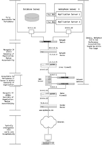
Figure 6-1: An end-to-end measurement
You'll need to understand and determine whether your testing is conducted from a response time perspective (from the Web server to the database server) or whether it encompass the transfer time from the user all the way through backend (for example, the database). This is important to determine your requirements. Are you spending too much time trying to improve the performance of something you can't control (for example, the Internet), or should you focus on the things within your control, such as the WebSphere application server and the database server?
My recommendation is stick with the things that are in your "circle of influence." However, you should be at least aware of the big picture. It's important to ensure that all elements are included or considered with your performance methodology. Get the right people with the right skills involved with your tuning efforts, especially in areas of your environment with which you may not be 100 percent comfortable.
In your optimization strategy, you may decide that you want to go down a level or two and state that different tiers must have certain response times. This would be typical for larger environments where there are a mix of asynchronous type transactions going off to legacy mainframe systems or batch and report runs that may take several hours to complete while providing online, interactive response times for real-time data.
Consider elements such as firewalls, load balancers, switches, and other infrastructure- related items that may not be in your direct control but that affect your WebSphere application's overall performance. There can be hundreds of components within an enterprise-class WebSphere environment that'll need to operate efficiently for a WebSphere application to perform well.
Many of these components, such as firewalls and switches, are beyond the scope of this book. However, this shouldn't discourage you from including them in your plan for overall platform optimization. You, as the application or system manager, need to set expectations for these aspects of your platform's performance.
In Figure 6-1, there are scope guides on the left side, which indicate the boundary of accountability in terms of managing response times. What the figure is attempting to show is the different areas within your WebSphere environment and a breakdown via the scope guides as to who or what is in "scope" for end-to-end response time accountability. Obviously, if in your organization you're only responsible for managing the immediate WebSphere environment systems, you may have little area of influence in the design and performance of the firewall. Then again, you may be working for a smaller organization where you're responsible for more than just the WebSphere environment and may in fact also have accountability for the firewall and network components!
Concurrent and Registered Users
How many users will be using your application environment (for example, how many registered users?), and how many will be concurrently using the application? There's a big difference between the two, and it's one I have to explain often.
Your application may have one million registered customers, but you may be providing a service that only sees them using the application once per year. Therefore, your concurrent user count is low. You can work out or at least surmise what your approximate concurrent user rate will be by understanding the operational hours and the frequency of usage.
For example, if your application is open 24 —7 but is only used during normal business hours local to your time zone, you can infer that, based on ten- hour days for a week, you should expect approximately 45 concurrent users based on a ten-minute session time. This isn't much at all and could be easily handled by the most modest of WebSphere installations.
On the other hand, if you expect your registered user base of one million customers to use the application daily, then the figures look a lot different. The resulting load would be an approximate 165,000 concurrent users online at any one time, and the WebSphere environment to match would give any hardware enthusiast a level of adrenalin!
Sure, these are extreme cases, but they do happen; I've seen both ends and all points in the middle.
Transaction Characteristics
You can further spread that spectrum of user load in the previous section. What if those 165,000 concurrent users were using the WebSphere-based platform to simply obtain an account balance for their savings account? This would infer a fairly lightweight transaction characteristic.
The other end of the spectrum would be if all users, in both scenarios, were coming to perform online tax returns. This would be a heavyweight transaction characteristic per session, given the amount of underlying logic that would be needed. All the checks and balances , the storing, the validation, and the dynamic presentation based on user input are examples of the business logic that would be included in a system such as this.
In earlier chapters, I touched on the topic of transaction characteristics and how you'd model with them. As mentioned, a transaction characteristic has more of an impact on a system's response time and load than does the number of users using the application environment. The only paradox is that it takes users to drive the transaction characteristic effect, not the other way around.
However, if you were to graph different levels of concurrent users using a system against differing levels of transaction characteristics (for example, low, medium, and high), then this transaction characteristic effect would be far more profound. Another way to look at this is this: If you have a lightweight transaction-based system, had 20 users concurrently online, and tested 40, then 80, and then 160, then you'd probably see the utilization graph of the overall environment increase quite smoothly if your system was able to handle the increase in concurrent users to 160.
However, if you performed the same test, with the same amount and increasing number of concurrent users on a system that had heavyweight transactions, you'd quickly see the system start to be affected far more than that of the lightweight transaction-based system.
To explain this further, Figure 6-2 shows lightweight versus heavyweight transactions.
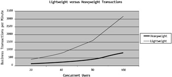
Figure 6-2: Lightweight versus heavyweight transaction characteristics
As you can see from Figure 6-2, the first test with the light line is the lightweight transaction test, and the other test, the heavyweight transaction, is in the darker color . The left axis is the total number of transactions at each level, and the horizontal axis is the number of users online.
As you can see, the lightweight transactions are increasing at a far faster rate than the heavyweight transactions. This seems somewhat obvious, but you need to understand that one of your expectations is that you're aware of and know what the transaction characteristic of your application environment is.
The reason for the transaction characteristic to be higher in a lightweight transaction environment is that heavyweight transactions are just that ”they're heavy (in other words, they take up more system resources). The heavier the weight of the transaction, the more effort and processing power is required within the environment.
Transaction Rate
Not completely separate but definitely different from the transaction characteristic expectation is the transaction rate. Transaction rate is almost a reverse of what you just looked at. It's another way of understanding what the load of your application may look like.
Transaction rate plus transaction characteristic equals your transaction profile. That is, it determines how many transactions your users will be performing on the WebSphere platform when they use the system. If they're logged in for, let's say, ten minutes at a time, they may perform five clicks.
Those five clicks drive the number of transactions. Within your environment, you need to understand how many function transactions (user clicks) take place per user and per session and, of those function transactions, what the underlying application transactions are that take place.
Remember that if your Web-based User Interface (UI) is made up of not only dynamic content ”driven by JavaServer Pages (JSP) or Hypertext Markup Language (HTML) ”but also many images such as JPEGs and GIFs, then this will increase the time to display your UI. For example, displaying one 200-kilobyte (KB) image displayed within a Web UI will be faster than displaying ten 25KB images. The more images and components you have within your UI, the more interactions occur between the user browser and the Web or application server.
The perceived response time for displaying a Web UI increases as the bandwidth between the user's browser and the Web or the WebSphere server decreases in capacity. This is important to remember when designing and tuning your presentation framework ”consider a best fit rather than trying to tune for all specific bandwidth types.
Of course, if you're implementing a WebSphere application purely for Local Area Network (LAN) or even high-speed broadband users, then your job is easier. The effects of the multiple page "component composition latency" on broadband or LAN speed networks can be somewhat masked because of the high speed of the networking medium.
| Note | Don't get mixed up between Java/J2EE transactions and the transactions I'm talking about in this chapter. They're two separate concepts and unfortunately are commonly misunderstood! |
Consider this example of transaction rate: If your users or customers are using the application to look up movie times, this could be perceived as having a fairly low transaction rate. The user logs in (one functional transaction), chooses the date they'd like to see a film (one functional transaction), selects the cinema of choice (a one functional transaction), reads a synopsis (one functional transaction), and then logs out (one functional transaction). There are four functional transactions. Therefore, the functional transaction rate per customer is an average of four per session.
But what happens under the hood? Each of those functional transactions may have to perform complex database queries, validation against the user profiles to make sure they're able to view synopses of movies allowable for their age group (for example, the G, PG, PG-13, and R ratings), and so forth. Each of these transactions may average to be five application transactions per functional transaction. This would lead to an average of 20 application transactions per user session (in other words, four functional transactions multiplied by the number of application transactions, which equals 20).
The expectation you need to consider here is the number of transactions taking place, both as an average functional transaction and as an average application transaction. These figures will help you build up a performance profile of your application ”one that will help you better model for future capacity.
You'll look at profiling and benchmarking in more detail during Chapter 15.
Application Availability
Although application availability is a service level in itself, it's not a performance measurement per se. It may be deemed a performance "yardstick" in the context of a contractual agreement or legal binding between a developer and a company, but, at the face of it, it's not directly in the path of system performance.
However, I've seen application availability cause an impact on the performance of an application in the case of buggy software or unstable hardware. Imagine for a minute that you have a complex application environment with several database nodes running in a High Availability (HA) cluster. For some reason, the clusterware is unstable and is causing the database nodes to failover to one another.
Given that an HA database may take up to a minute to failover to one of its constituent nodes, this will result in a decreased transaction rate potential, and therefore, overall performance will be lowered (with performance measured by the number of transactions per minute or per second).
The Outcome: Measuring Your Expectations
Once you've determined what your expectations are, you need to understand how you're going to test. I also touched on this point back in Chapter 1, and it's an age-old problem with performance modeling, monitoring, and analysis. Quite often, your testing will drive load onto your application. How are you going to test your WebSphere application so that you cause as little impact on it as possible? It's almost impossible to do any form of monitoring without impacting your customers or users.
As soon as you implement user experience monitors (in other words, test harnesses that access key function points of the WebSphere-based application and time the result speed), you impact your overall application environment. The impact may only be small, but it's still an impact, and your results are skewed (albeit, potentially only a small amount).
One method to avoid this is to build into your application response time monitors. This way, each transaction will be timed, and there will be no impact to your perceived application response time because the small overhead associated with the extra application timing code will be considered "business as usual" for your application.
Therefore, you need to define the method of monitoring and testing that both suits your specific application and that provides you with the best results in terms of being able to match them against your expectations.
The following are some words of wisdom:
-
Don't write timing markers into your code and output them to the WebSphere standard out (in other words, <WebSphere_HOME>/logs/ <application_name>. stdout .log ) or standard error (in other words, <WebSphere_HOME>/logs/<application_name>.stderr.log ) logs if you're trying to achieve a fine level of optimization. I've seen this being done a lot. Although it's probably safe to use this form of logging once for analysis or for specific debugging tasks (rather than for performance management), running these types of timer outputs can skew your results. An incorrect implementation of the custom-built timer class may be single-threaded in nature, and as such, the whole application has to wait for it to complete assigned time stamps to variables . Although this may not impact a small application with only a handful of customers or users online, if every user had to wait 300 milliseconds for a static thread to complete on a 500 concurrent user system, it'd slow the overall performance down considerably.
-
Be aware that different operating systems have different timing resolutions when using standard Java timing classes. This resolution variance can be as much as 15 milliseconds (ms) for Windows-based applications.
-
Do consider placing time stamps in logging entries within your database. This can incur a small amount of overhead, but far less than that of the previous item. In this case, you'd schedule weekly or nightly jobs to run through the database and run a report the various time stamp and thread ID combinations. For example:
SQL> select txn_entry_type from operational_log_t where txn_entry_type ' START' and 'STOP';
 -
Although this puts load on the database during the report time, you can schedule the task to run during off-peak or nonoperational periods.
-
Another design consideration in using this approach is to cache the timing figures into some form of memory or cache storage area and periodically persist the information to the database. If you have 5,000 concurrent users with hundreds of page clicks per second, your database will be quickly consumed with timing data inserts rather than serving customer- facing application requests .
-
You may want to consider using the Performance Management Interface (PMI) timing hooks available within the WebSphere application server. These interfaces allow you to access various timing measurements and can avoid overheads associated with issues such as the one mentioned previously (database insertion overhead). You'll look at PMI in Chapter 13.
-
Do operate user experience monitors. That is, use any number of the product suites on the market that allow you to simulate a user using the various key functions of an application.
-
This does increase load by a factor indexed against the frequency of the test and what sort of functional tests are involved; however, given the test is testing live functionality, you should have an idea from your initial setting of expectations what the impact will be. Therefore, you could run the test and extrapolate backward, calculating for the discrepancy of the test user.
-
Don't run technical tests behind the scenes unless you really must. That is, don't run scripts that periodically hit the database or specific methods within the application from the command line or batch-driven processes that "probe" certain aspects of the application. If you do, you'll need to make sure you compensate for the load you're introducing. You'll need to be careful that you don't skew your results by not following through on a complete business transaction. For example, if you're trying to hit a method within an Enterprise JavaBean (EJB) Java Archive (JAR) that will time the response to query all movie sessions at a particular cinema, your transaction test may not factor in predecessor variables that might be applicable when the true transaction is executed by a real live user or customer. For example, what if your test is simply hitting a null field in order to obtain method invocation and execution time. However, although this may give a result of "x," the true value of "x" may be quite different when you obtain "x" through a live transaction (for example, session setup, presentation tier delays, and so on).
-
Do baseline your WebSphere-based application in a controlled and scientific manner. Baselining and profiling are your friends when it comes to performance optimization. They're the key performance (no pun intended) indicators that'll determine if the optimization approach you're performing is working. In Chapters 13 and 14 you'll look at the tooling and baselining of WebSphere and WebSphere-based J2EE applications.
Although this isn't an exhaustive list, the basic premise is that monitoring and testing application software impacts the net response curve for all users. Table 6-1 summarizes the various testing types.
| Monitoring Type | Test Accuracy | Potential Impact to Performance | Overall Test Result Quality |
| Intrusive probes | Medium | High | Low |
| Method timings output to logs | Medium | Medium | Medium |
| Database reports based on transaction time markers | High | Low | Medium |
| User experience monitors | High | Medium | High |
As you can see, the best result of testing is a true user or customer simulation test. It provides an overall test result that gives accurate performance indicators for the testing that you're trying to achieve. It doesn't, however, provide an ability to test each specific method of interface during the overall user session without more sophisticated software.
I'll discuss this in more detail in Chapter 14.
Tools for Testing
With all the discussion about what to test and how to test it, it's worth discussing what tools are good for testing your WebSphere environment.
Essentially, you can break down testing tools into three main groups:
-
Profilers and benchmarkers
-
Monitors and probes
-
Stress and volume suites
The following sections explain each of these.
Profilers and Benchmarkers
This group of testing tools builds a baseline of your application's performance. Typically these are used before and after optimizing as part of your strategy.
For WebSphere, there are a number of free, open-source, and commercial profilers that help with this. Table 6-2 summarizes some of the tools that work well with WebSphere-based environments. Again, this list isn't exhaustive, but it includes tools I've found to work well within WebSphere-based environments. The table provides an overview of the various packages, and I'll discuss their use and implementation in more detail in Chapter 14.
| Tool/Application | License Availability | Tool Type |
|---|---|---|
| Grinder | Open source | Profiling and load testing |
| WinRunner, Mercury Interactive | Commercial | Profiling and load testing |
| Jprobe, Quest Software | Commercial; demo availale | Profiling |
| HPJMeter, Hewlett-Packard | Freely available download | Profiling |
| Custom-built packages using operating system tools | Included in your operating system | Profiling |
I've provided links to these software packages in Chapter 14. All of these applications provide value on their own; however, WebSphere comes with a Resource Analyzer package that allows you to monitor the operational aspects of your applications.
Resource Analyzer includes features such as the number of active threads, the number of connections, the number of sessions, the number of EJB cache hits, and so on. All these tools will help to provide a picture for the operational status of your application, as well as give you a good understanding of the state of your application under certain loads (for example, during load testing or during normal operational production load).
Monitors and Probes
Monitors and probes are typically associated with operational alarming and the likes. For example, you may have a specific function that needs to be regularly tested (probed) to see that its response time doesn't exceed "y" number of seconds.
The monitors may also be a way to understand availability and uptime of your components. That is, how often does a Java Virtual Machine (JVM) crash or how often does a JVM garbage collect? The latter will definitely impact the overall performance of your application. If you're able to monitor and plot this, you may be able to identify a trend in your WebSphere-based applications, such as too little heap space.
You can find some of the most useful monitoring packages in the open-source arena. Furthermore, a range of commercial products allow you to feed information from WebSphere into them. You may also be at a site that has an enterprise systems management suite that you're able to hook into.
Table 6-3 describes some common tools that are useful as monitors and probes.
| Tool/Application | License Availability | Tool Type |
|---|---|---|
| Multi Router Traffic Grapher (MRTG) | GNU/open source | Monitoring tool (Graphing) |
| RRDtool | GNU/open source | Monitoring tool (Graphing) |
| Lynx | GNU/open source | Command line Web browser with some nifty features |
| Curl | GNU/open source | Powerful command line tool for probing Internet services |
| Custom-built Java applications | Provide any form of analysis and monitor desired | |
| Big Brother | Open source/commercial | Monitoring and alerting |
I tend to use these packages a lot given that they're open source and readily available. Again, you'll look at their implementation in later chapters.
Stress and Volume
Stress and volume testing is a bit of a science. It's not as simple as running a while true loop and pounding away at an application for a designated time-frame. Many commercial offerings exist in this field, and all of these are sophisticated software application suites, capable of everything from simple stress and volume testing to ongoing capacity and resource management facilities.
It should be a golden rule that prior to any production system going live, formal stress and volume testing should be undertaken. When conducted properly and at the right stage during software development, stress and volume testing will help both the developers and architects identify if there are any hot spots or bottlenecks within the application and, more importantly, how the application operates under load and volume.
I'll briefly discuss what stress and volume testing is. Stress testing is a test to identify whether there are any issues with the application or platform when a level of computational or derived load is placed on the aforementioned components. This is different to volume testing , which tries to identify what the upper limits are in terms of resource utilization from a volume perspective.
For example, volume testing checks to see how many concurrent transactions a particular (or a whole) component will be able to handle. For example, you may want to volume test your database connections from your WebSphere environment to understand how many concurrent queries can be sustained before the performance and response times of those queries go beyond your expected results.
Stress testing is more of a peak load test. If you have two WebSphere application servers operating and one of them crashes, requiring the remaining application to server to take over the load, will the secondary server be able to handle the additional peak load, or the stress, of double the connections all within a short period?
Ninety-five percent of the time, you'll conduct stress and volume testing together. If your application is large and complex and has countless components, you'd want to test specific components and elements in specific ways.
Table 6-4 shows some of the stress and volume tools available.
| Tool/Application | License Availability | Tool Type |
|---|---|---|
| LoadRunner, Mercury Interactive | Commercial | Stress and volume testing |
| Microsoft Web Application Stress Tool | Free | Stress and volume testing |
| PerformaSure, Quest | Commercial | Stress and volume with application management |
| Curl/Perl/Lynx | GNU/open source | Combination of software to help custom build stress and volume testing suites |
| Custom-built packages | Custom built to your site's requirements |
Stress and volume testing is a complex area of operational architectures and software delivery. It's a science within itself, and there are many books dedicated to the planning of stress and volume testing.
You'll learn how to best test WebSphere and WebSphere-based applications using stress and volume testing methodologies that'll focus on planning and understanding what you want to test and then map those expectations to a plan to achieve your desired testing outcomes .
Measuring the Effects of Tuning
Recording the results of testing is just as important as testing is. Most of the commercial packages have plotting and data presentation tools that allow you to make graphics and historic models of the testing. Some of the other software, such as those from the open-source industry or under the General Public License (GPL), needs to have its results interpreted by something. This is especially the case when you develop your own probes and tests, which simply output numerical data that, on its own, presents no information at all.
My preference for occasional graphing or plotting is to use a spreadsheet program such as Microsoft Excel. These types of spreadsheet applications provide an enormous amount of mathematical facilities for plotting and analyzing all kinds of data. With Microsoft Excel, you're able to plot and analyze almost any form of input data you can think of, and you can correlate any number of data types within a single graph.
If, however, you're keen to use automated tools that run from your Windows scheduler or a Unix Cronjob, applications such as MRTG and RRDtool provide great solutions. Both of these products are the creation of Tobias Oetiker, and both are high quality and fast. In the case of RRDtool, it's a very powerful graphical plotting application.
| Note | You'll look at MRTG and RRDtool in more detail in Chapter 13 and 14. |
However, part of the process of performing optimizing and tuning on a WebSphere-based application environment is being to plot and determine the results. Further, if you're six months into an operational cycle within a WebSphere-based environment, you should have continued monitoring and probing occurring against your application environment. The reason for this is so you can build up both a historic reference and a model for growth. The historic reference is a safeguard to help ensure that you have a clear view, with historic perspective, of any trend for the component of your environment you're monitoring.
A classic usage for this type of monitoring is network utilization. Over time, theoretically, if your application is increasing in load and usage (usually driven by additional functionality, bug fixes, and so on), you'll have a situation where your network traffic will also be increasing.
Like most things in the computing world, networks of any size have limitations on their capacity, and, with the increase in load, there will be an increase in network utilization. Using a combination of a network interface monitor (which could be something as simple as a netstat -i command periodically outputting to a text file or an snmpget command on your network interface) and a graphing or plotting tool such as MRTG or RRDtool, you'll see an increase in usage over time.
Some additional scripts could output the results of the netstat -i command or snmpget command to a centralized alerting tool for operator notification.
A common test I implement to monitor WebSphere JDBC connection pool usage is an external Perl script that, using Perl DBI modules, periodically logs into various databases and understands how many and which users are logged in. With this, I know how many times a specific user is logged in and plot that against how many user logins there should be. I can correlate that with the WebSphere JDBC Resource settings ”via either an XMLConfig dump or WebSphere Control Program (WSCP) output for WebSphere 4 or wsadmin output in version 5 ”to determine whether I'm close to the threshold.
Figure 6-3 shows an example of what the output of a database connection script would look like, once plotted.
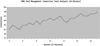
Figure 6-3: Database connection usage
Quite clearly, you can see the trend is increasing over time for the JDBC connection pool usage. If you had the JDBC connection pool maximum connections set to 50, the graph would clearly show that the JDBC provider is about to hit its upper limit and exhaust all available pooled connections (not a good thing).
| Note | You'll walk through creating these types of scripts later in Chapters 13 and 14. |
In this example, the trend is suggesting some sort of code-related problem with not closing off connections to the database. As you can see in this figure, the number of connections is slowly increasing over time, somewhat analogous to a memory leak. Although this upward trend of increasing connections to the database may simply be that of an organic increase in connection load (in other words, as load increases toward peak periods), these sorts of trends invariably lead to code-related problems.
Either way, historic trend analysis is important when already operating a WebSphere application environment and while conducting an optimization strategy.
In the case of the optimization strategy, your time frame or historic data will be compressed and therefore will more likely result in profiling or baselining runs. For example, let's say you're attempting to tune a JVM for an application server operating on a WebSphere platform.
The initial settings for the JVM may be set at 768MB of the initial heap and 1024MB for the maximum heap size. If your application environment is under constant load, it's best to set the minimum and maximum JVM heap sizes to be the same. In my experience, it's better to set these values the same in a high-load environment, slightly higher than what you may actually require, to avoid garbage collection.
As discussed several times in the book so far, garbage collection is a heavy hitter for overall application performance degradation in Java/J2EE environments. Your garbage collection is believed to be occurring too frequently, so let's assume you've attempted to look at this problem by analyzing the output in the standard WebSphere application server log file (a standard out file).
| Tip | In order to obtain verbose garbage collection output from your JVM, you'll need to include the -verbosegc directive in your JVM startup parameters. |
If you were to watch the log files for this example JVM, you may see some garbage collection occurring via the following types of output messages:
[GC 983301K->952837K(1021216K), 0.0207301 secs] [GC 983301K->952837K(1021216K), 0.0222956 secs] [GC 983301K->952837K(1021216K), 0.0234131 secs] [GC 983301K->952837K(1021216K), 0.0246168 secs] [GC 983301K->952837K(1021216K), 0.0230762 secs] [GC 983301K->952837K(1021216K), 0.0222828 secs]
This output, from a Sun Solaris JVM, is indicating a line for every JVM garbage collection occurring for your specified application server.
| Note | Other platform JVM garbage collection output will vary slightly. Generally, they'll exhibit the same amount of basic information. |
The first column after the [GC is the amount of heap space allocated prior to garbage collection. The second field is referring to the amount of memory allocated after garbage collection has taken place. The number in parentheses is the currently allocated heap, which in this case is 1,024 megabytes (MB), or 1 gigabyte (GB), of memory.
| Tip | If your system has Grep, Sed, and Awk installed ”such as all Unix servers ”the following command will allow you to quickly obtain garbage collection information from your log files: grep / awk '/^<GC/ {print ($12); }' sed "1,\$s/>//" . |
The last number in the previous code is the time taken for the cleanup to occur. As you can see in this example, the time taken is relatively small; however, what's not shown here is the time between collections.
This data by itself isn't too useful. You may get a feeling that there's excessive cleanup occurring if you see either large cleanup amounts (greater than 50 percent of the heap) or that the time taken to clean up is longer than one second.
However, if you're analyzing a performance problem and trying to log that there may be errors, you can't beat good historic reference data.
The previous numbers provide data but not information. If you were to graph that data, you'd see something like Figure 6-4.
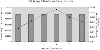
Figure 6-4: Example logging of garbage collection
As you can see, Figure 6-4 shows a fairly uninteresting story. There's neither a linear reference nor anything to correlate it with (for example, no load or utilization indices to indicate if the system was under load).
If, on the other hand, you had collected the garbage collection information over time, Figure 6-5 shows what you can infer from good data.
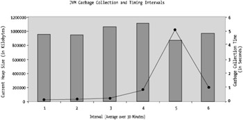
Figure 6-5: Historic garbage collection logging
As you can see, there are some pretty significant cleanup points in Figure 6-5 that indicate some heavy object utilization. This may not be necessarily a problem in itself; however, given that the heap is nearly 100 percent allocated for a good proportion of the time, it's definitely worth looking at the object utilization and even the amount of heap allocated to this JVM.
EAN: 2147483647
Pages: 111