12.2 Software Reliability
|
|
12.2 Software Reliability
There have been many attempts made to understand the reliability of software systems through software reliability modeling. These models have become very sophisticated. They are able to predict the past with great accuracy. Unfortunately, these models are essentially worthless for predicting the future behavior of software systems. The reason is really quite simple; most attempts to understand software reliability have attempted to model software in exactly the same manner as one would model hardware reliability. Herein is the nut of the problem. Software and hardware are vastly different.
A hardware system is an integrated and functional unit. When a jet engine, for example, is running, all of the pieces of this jet engine are involved in the process of generating fire and great mayhem. Similarly, when a new computer CPU chip is energized, the whole surface of the chip is engaged in directing the flow of electrons. Further, when either of these systems is manufactured, there will be slight differences in them as a result of the manufacturing process. If nothing else, the atoms that comprise any two CPU chips are mutually exclusive.
Software systems are very different. The control software for a cellular telephone is exactly the same for each telephone set. All telephones with the same release of software will have exactly identical software loads on them. There is exactly zero manufacturing variation in these systems. If there is a fault in one software system, then that same fault will be present in all systems.
Just as a CPU chip has thousands of component parts, so will an equally complex software system. In a CPU chip, all of these systems are working at once. In our software system, only one component is operational at any instant. This is a phenomenally important difference. A software system is not the sum of its parts; it is only its parts. Some of these parts are more flawed than others.
The failure of a software system as it is dependent only on what the software is currently performing: operations that a user is performing. If a program is currently executing an operation that is expressed in terms of a set of fault-free modules, this operation will certainly execute indefinitely without any likelihood of failure. Each operation causes a program to execute certain program modules. Some of these modules may contain faults. A program may execute a sequence of fault-prone modules and still not fail. In this particular case, the faults may lie in a region of the code that is not likely to be expressed during the execution of a function. A failure event can only occur when the software system executes a module that contains faults. If an operation is never selected that drives the program into a module that contains faults, then the program will never fail. Alternatively, a program may well execute successfully in a module that contains faults just as long as the faults are in code subsets that are not executed.
Some of the problems that have arisen in past attempts at software reliability determination all relate to the fact that their perspective has been distorted. Programs do not wear out over time. If they are not modified, they will certainly not improve over time, nor will they get less reliable over time. The only thing that really impacts the reliability of a software system is the operations that the program is servicing. A program may work very well for a number of years based on the operations that it is asked to execute. This same program may suddenly become quite unreliable if the user changes its mission.
Existing approaches to the understanding of software reliability patently assume that software failure events are observable. The truth is that the overwhelming majority of software failures go unnoticed when they occur. Only when these failures disrupt the system by second-, third-, or fourth-order effects do they provide enough disruption for outside observation. Consequently, only those dramatic events that lead to the immediate collapse of a system can be seen directly by an observer when they occur. The more insidious failures will lurk in the code for a long interval before their effects are observed. Failure events go unnoticed and undetected because the software has not been instrumented so that these failure events can be detected. In that software failures go largely unnoticed, it is presumptuous to attempt to model the reliability of software based on the inaccurate and erroneous observed failure data. If we cannot observe failure events directly, then we must seek another metaphor that will permit us to model and understand reliability in a context that we can measure.
Computer programs do not break. They do not fail monolithically. Programs are designed to perform a set of mutually exclusive tasks or functions. Some of these functions work quite well while others may not work well at all. When a program is executing a particular function, it executes a well-defined subset of its code. Some of these subsets are flawed and some are not. Users execute varying subsets of the total program functionality. Two users of the same software might have totally different perceptions as to the reliability of the same system. One user might use the system on a daily basis and never experience a problem. Another user might have continual problems in trying to execute exactly the same program. The reliability of a system is clearly related to the operations that a user is performing on the system.
Another problem found in software reliability investigations centers on the failure event itself. Our current view of software reliability is colored by a philosophical approach that began with efforts to model hardware reliability (see Musa [1]). Inherent in this approach is the notion that it is possible to identify with some precision this failure event and measure the elapsed time to the failure event. For hardware systems this has real meaning. Take, for example, the failure of a light bulb. A set of light bulbs can be switched on and a very precise timer started for the time that they were turned on. One by one the light bulbs will burn out and we can note the exact time to failure of each of the bulbs. From these failure data we can then develop a precise estimate for both the mean time to failure for these light bulbs and a good estimate of the variance of the time to failure. The case for software systems is not at all the same. Failure events are sometimes quite visible in terms of catastrophic collapses of a system. More often than not, the actual failure event will have occurred a considerable time before its effect is noted. In most cases it is simply not possible to determine with any certainty just when the actual failure occurred on a real-time clock. The simplest example of this improbability of measuring the time between failures of a program can be found in a program that hangs in an infinite loop. Technically, the failure event happened on entry to the loop. The program, however, continues to execute until it is killed. This may take seconds, minutes, or hours, depending on the patience and attentiveness of the operator. As a result, the accuracy of the actual measurement of time intervals is a subject never mentioned in most software validation studies. Because of this, these models are notoriously weak in their ability to predict the future reliability of software systems. A model validated on Gaussian noise will probably not do well in practical applications. The bottom line for the measurement of time between failures in software systems is that we cannot measure these time intervals with any reasonable degree of accuracy. This being the case, we then must look to new metaphors for software systems that will allow us to model the reliability of these systems based on things that we can measure with some accuracy.
Yet another problem with the hardware adaptive approach to software reliability modeling is that the failure of a computer software system is simply not time dependent. A system can operate without failure for years and then suddenly become very unreliable based on the changing functions that the system must execute. Many university computer centers experienced this phenomenon in the late 1960s and early 1970s when there was a sudden shift in computer science curricula from programming languages such as FORTRAN that had static runtime environments to ALGOL derivatives such as Pascal and Modula that had dynamic runtime environments. From an operating system perspective, there was a major shift in the functionality of the operating system exercised by these two different environments. As the shift was made to the ALGOL-like languages, latent code in the operating system, specifically those routines that dealt with memory management, that had not been executed overly much in the past now became central to the new operating environment. This code was both fragile and untested. The operating systems that had been so reliable began to fail like cheap light bulbs.
Each program functionality can be thought of as having an associated reliability estimate. We may choose to think of the reliability of a system in these functional terms. Users of the software system, however, have a very different view of the system. What is important to the user is not that a particular function is fragile or reliable, but rather whether the system will operate to perform those actions that the user will want the system to perform correctly. From a user's perspective, it matters not, then, that certain functions are very unreliable. It only matters that the functions associated with the user's actions or operations are reliable. The classical example of this idea was expressed by the authors of the early UNIX utility programs. In the last paragraph of the documentation for each of these utilities there was a list of known bugs for that program. In general, these bugs were not a problem. Most involved aspects of operation that the typical user would never exploit.
The main problem in understanding software reliability from this new perspective is getting the granularity of the observation right. Software systems are designed to implement each of their functionalities in one or more code modules. In some cases there is a direct correspondence between a particular program module and a particular functionality. That is, if the program is expressing that functionality, it will execute exclusively in the module in question. In most cases, however, there will not be this distinct traceability of functionality to modules. The functionality will be expressed in many different code modules. It is the individual code module that fails. A code module will, of course, be executing a particular functionality associated with a distinct operation when it fails. We must come to understand that it is the operation — not the software — that fails.
We will see that the key to understanding program failure events is the direct association of these failures to execution events with a given operation. A stochastic process will be used to describe the transition of program modules from one to another as a program transitions among operations. From these observations, it will become fairly obvious just what data will be needed to accurately describe the reliability of the system. In essence, the system will be able to apprise us of its own health. The reliability modeling process is no longer something that will be performed ex post facto. It can be accomplished dynamically while the program is executing. It is our goal to develop a methodology that will permit the modeling of the reliability of program operation. This methodology will then be used to develop notions of design robustness in the face of departures from design operational profiles.
12.2.1 Understanding Software
Computer software is very different from the hardware on which it resides. Software is abstract whereas hardware is real and tangible. There is nothing to suggest that software artifacts share any common attributes with their hardware counterparts, save that they were both created by people. It is unrealistic to suppose that any mathematical modeling concepts that apply to hardware development would relate to software. Consider the case, for example, of the manufacture of pistons for automobile engines. Each piston is uniquely different from its predecessor and its successor on the manufacturing line. Each piston has metallic elements that are not shared with any other piston. Further, the metallic composition of each piston is slightly different from every other piston. Each piston is slightly different in its physical size and shape from its neighbors. We can characterize these differences in degree by the statistical notion of variance. The pistons are designed to an average or expected value and the manufacturing processes then approximate this design value. A good manufacturing process is one that will permit only very small variations in the actual physical and chemical properties of the pistons.
In the manufacture of embedded software systems, there is zero variance among production software systems. If there is a fault in the control software for a single cell phone, then this defect will be present in every cell phone manufactured that contains this particular software release. They will all be flawed. If there is a software fault in the new release of a popular operating system, all of the software systems of that release will be flawed. They are all identical. There is zero variance. In essence, when we construct software, we build only one system, ever. There may be many copies of these systems but they are all perfect clones. Thus, the basic principles of statistical quality control simply do not apply to manufactured software systems.
The manner in which software systems will be used when they are deployed, however, does vary. This means that each user of the system will, in fact, be using a different software system. They will, by their operational profiles, select certain subsets of the code to exercise in ways that do vary from one user to another. Thus, our statistical models must reflect the context of the use of the software and not the software system itself. The variance in the software system is induced by the context and is not an intrinsic property of the software.
Physical systems also change with respect to time. Components that move over each other will cause wear and abrasion. Electrical current anomalies will gradually erode the chemical substrate of integrated circuits. Software systems, on the other hand, do not change with respect to time. They are eternal. They quite literally operate in a different universe than the one we occupy. The software universe is devoid of space and time. There is no such thing as gravity. In essence, different rules of physics apply in this timeless universe. Our success in understanding software is predicated on our ability to formulate mathematical models of behavior consistent with the physics of this different universe.
12.2.2 Software Reliability Modeling
It is increasingly evident that the reliability of a software system is largely determined during program design. One distinct aspect of the software design process that lends itself to measurement is the decomposition of the functionality of a system into modules and the subsequent interaction of the modules under a given set of inputs to the software. The actual distribution of execution time to each software module for a given input scenario is recorded in the execution profile for the system. For a given input scenario to a program, the execution profile is a function of how the design of the software has assigned functionality to program modules.
The reliability of a software system can be characterized in terms of the individual software modules that make up the system. From the standpoint of the logical description of the system, these functional components of the larger system are, in fact, operating in series. If any one of these components fails, the entire system will fail. The likelihood that a component will fail is directly related to the complexity of that module. If it is very complex, the fault probability is also large. The system will be as reliable as its weakest component.
For each possible design outcome in a software design effort, there will be a set of expected execution profiles, one for each of the anticipated program functionalities. We should evaluate design alternatives in terms of the variance of functional complexity. If there is high variability in functional complexity, the reliability of the product of the design is likely to be low. A reasonable design objective would be to reduce functional complexity.
At the design stage, quantitative measures correlated to module fault-proneness and product failure provide a means to begin to exert statistical process control techniques on the design of a software system as an ongoing quality control activity. Rather than merely documenting the increasing operational complexity of a software product and therefore its decreasing reliability, one can monitor the operational complexity of successive design adaptations during the maintenance phase. It becomes possible to ensure that subsequent design revisions do not increase operational complexity and especially do not increase the variance among individual module's functional complexity.
It is now quite clear that the architecture of a program will be a large determinant of its reliability. Some activities that a program will be asked to perform are quite simple. Designers and programmers alike will easily understand them. The resulting code will not likely contain faults. If, on the other hand, the specified functionality of a program is very complex and as a result ambiguous, then there is a good likelihood that this functionality will be quite fragile due to the faults introduced through the very human processes of its creation. A more realistic approach to software reliability modeling will reflect the software reliability in terms of the functionality of the software.
12.2.3 Software Module Reliability
To capture the essence of the concept of software failure, let us suppose that each software system has a virtual failure module (VFM), mn+1, to which control is automatically passed at the instant the program departs from its specified behavior. We can easily accomplish this action with assertions built into the code. In essence, we cannot perceive a failure event if we are not watching. Some program activities such as a divide by zero will be trapped by the system automatically. The hardware and operating system, however, cannot know our intentions for the successful execution of a module on a more global scale. We must instrument the code to know whether it is operating correctly. Programming assertions into the code is a very good way to measure for failure events.
There are really three levels of granularity of program reliability. At the lowest level of granularity, there is module reliability. The module design process has specified each program module very carefully. We know what it should be doing. We can easily define the parameters for its successful operation. We can know, that is, whether the program module is operating within its design specifications. The moment that it begins to operate outside its design framework, we will imagine that the module will transfer control to the VFM representing the failure state. Thus, if we have a system of n program modules, we will imagine that this system is augmented by a module that will trap all contingencies that arise when any program module has failed.
Each program module, then, will or will not fail when it is executed. We can know this and we can remember these failure events. A program module will be considered reliable if we have used it frequently and it has failed infrequently. A program module will be considered unreliable if we have used it frequently and it has failed frequently. A program module that has been used infrequently is neither reliable nor unreliable.
Any program module can transfer control to the VFM. This transfer, of course, can only happen if the current module has departed from program specifications. With our dynamic instrumentation and measurement technique, we can clearly count the number of times that control has been transferred to each module. Those data can be accumulated in a module execution frequency vector (MEFV). We can also count the number of times that control has been transferred from any module to the VFM. These data can be accumulated in a failure frequency vector (FFV) for each module. A module will be considered reliable if there is a small chance that it will transfer control to the VFM.
Let ti represent the ith element of the MEFV. It will contain the number of times that module i has received control during the last ![]() epochs. Similarly, let si represent the number of times that module i has transferred control to the VFM during the same time period. It is clear that si ≤ ti. That is, a module could have failed every time it was executed or it could have executed successfully at least once. Our current estimate for the failure probability of module i on the mth epoch is
epochs. Similarly, let si represent the number of times that module i has transferred control to the VFM during the same time period. It is clear that si ≤ ti. That is, a module could have failed every time it was executed or it could have executed successfully at least once. Our current estimate for the failure probability of module i on the mth epoch is ![]() . This means that of the total
. This means that of the total ![]() epochs that module i has received control, it has worked successfully on
epochs that module i has received control, it has worked successfully on ![]() epochs. The reliability of this module is simply one (1) minus its failure probability:
epochs. The reliability of this module is simply one (1) minus its failure probability: ![]() . From these observations we can construct a vector
. From these observations we can construct a vector ![]() of failure probabilities for each module on the mth epoch.
of failure probabilities for each module on the mth epoch.
It is clear that if module i has executed successfully for a large number of epochs, say 100,000, and failed but once over these epochs, then the module will be fairly reliable. In contrast, consider another module j that has executed only ten times and has not failed at all. At face value, the reliability of module j is 1, whereas the reliability of module i is 0.99999. However, we really lack enough information on module j to make a real accurate assessment of its behavior.
What we are really interested in is the current point estimate for reliability and a lower confidence for that estimate. It is clear that we can derive our estimate for the failure probability ![]() from
from ![]() . It is also clear that executing module i will have exactly two outcomes: it will execute successfully or it will fail. The distribution of the outcome of each trial will be binomial. Let us observe that for relatively large n, we can use the binomial approximation to a normal distribution with a mean of np and a standard deviation of
. It is also clear that executing module i will have exactly two outcomes: it will execute successfully or it will fail. The distribution of the outcome of each trial will be binomial. Let us observe that for relatively large n, we can use the binomial approximation to a normal distribution with a mean of np and a standard deviation of ![]() .
.
An estimate a for the (l - α)w upper bound for this failure probability can be derived from the binomial approximation to the normal distribution where:
![]()
If, for example, we wished to find the 9 percent confidence interval ![]() for
for ![]() , we could compute this from:
, we could compute this from:
where 1.65 is the x ordinate value from the standard normal (N(0,1)) distribution for α= 0.95. This estimate, ![]() , is an unbiased estimate for the upper bound of
, is an unbiased estimate for the upper bound of ![]() . The problem is that if we have executed a particular module only a very few times and it has not failed, then the number of failures
. The problem is that if we have executed a particular module only a very few times and it has not failed, then the number of failures ![]() for this module will be zero and the estimate for the upper bound
for this module will be zero and the estimate for the upper bound ![]() will also be zero. This would seem to imply that an untested module is also highly reliable and we are very confident about that estimate. Nothing could be further from the truth.
will also be zero. This would seem to imply that an untested module is also highly reliable and we are very confident about that estimate. Nothing could be further from the truth.
A more realistic assumption for the reliability of each module is to assume that it is unreliable until it is proven reliable. To this end, we will assume that each module has, at the beginning, been executed exactly once and it has failed. Thus, the number of measured epochs for each module will be increased by one and the number of failures experienced by that module will also be increased by one. Let ![]() and
and ![]() . Thus, a more suitable estimate for the initial failure probability for a module is
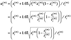
. Thus, a more suitable estimate for the initial failure probability for a module is ![]() with an upper bound on this estimate of:
with an upper bound on this estimate of:
![]()
We can construct a vector u(m) whose elements are the (1 - α) upper bounds on the estimates for the failure probabilities. Thus, with the vector of failure probabilities z(m) and the vector of upper bounds on these estimates u(m), we can characterize the failure potential and our confidence in this estimate of set of modules that comprise the complete software system.
As each functionality fi is exercised, it will induce a module execution profile ![]() on the set of n program models. That is, each functionality will exercise the set of program modules differently. Therefore, each functionality will have a different failure potential, depending on the failure probability of the modules that it executes. We can compute an expected value for the functionality failure probability of each functionality on the mth execution epoch as follows:
on the set of n program models. That is, each functionality will exercise the set of program modules differently. Therefore, each functionality will have a different failure potential, depending on the failure probability of the modules that it executes. We can compute an expected value for the functionality failure probability of each functionality on the mth execution epoch as follows:
![]()
In matrix form we can represent the vector of functional failure probabilities as q = pz(m), where p is an m × n matrix of module execution profiles for each functionality. We can also compute an upper bound on the expected value of the functional failure probabilities as q' = pu(m).
As each operation ωi in the set of l operations is exercised by the user, it will induce a functional profile ![]() on the set of k functionalities. That is, for every operation, there will be a vector of conditional probabilities for the execution of each functionality given that operation. Let p' represent the l × k matrix of the conditional probabilities of the k functionalities for the l operations.
on the set of k functionalities. That is, for every operation, there will be a vector of conditional probabilities for the execution of each functionality given that operation. Let p' represent the l × k matrix of the conditional probabilities of the k functionalities for the l operations.
It is clear that each operation will exercise the set of program functionalities differently. Therefore, each operation will have a different failure potential, depending on the failure probability of the functionalities that it executes. We can compute an expected value for the operational failure probability of each operation on the mth execution epoch as follows:
![]()
In matrix form we can represent the vector of operational failure probabilities as x = p'q, where p' is an l × k matrix of functional profiles. Substituting for q we can define x directly in terms of the measurable module failure probabilities to wit: x = p'pz(m). We can also establish an upper bound on the operational failure probabilities as x' = p'pu(m).
The elements of the vector x represent the failure probabilities for each of the l operations. The reliability of operation ωi can be derived from its failure probability as follows: ri = 1 - xi. Thus, we can construct a vector of operational reliability estimates r = I - x, where I is a vector of ones. We can also construct a vector of lower bounds on these reliability estimates: r' = I - x'.
The reliability of a software system is therefore not a static attribute of the system. It is an artifact of how the system will be used. There is a different reliability estimate for each operation, depending on how that operation exercises different modules. Furthermore, there is a lower bound on that reliability estimate, depending on how much we know about the modules that comprise that operation. A user's perception of the reliability of our system will depend on how he or she uses that system. The operational profile o represents the distribution of user activity across the system. Therefore, the user's reliability perception of the system ρ is simply ρ = or and the lower bound for this estimate is ρ' = or'.
12.2.4 Data Collection for Reliability Estimation
It seems pointless to engage in the academic exercise of software reliability modeling without making at least the slightest attempt to discuss the process of measuring failure events. A failure occurs immediately at the point that the program departs from its specification, not when we first perceive this departure. The latencies between when a system fails and when the user perceives this may be substantial. We could, for example, have a small memory leak in our Web browser. We will have to run this program for some time before it self-destructs, but die it will with this memory leak. The actual failure occurs at the point when the browser software failed to release some memory it had used. The instant when this first happened is when the failure occurred. If we are not watching, we will fail to see this happen. We will see it only when some functionality is first impaired. The user may not see the problem until the Web browser crashes or slows his machine to a crawl.
The basic premise of our approach to reliability modeling is that we really cannot measure temporal aspects of program failure. There are, however, certain aspects of program behavior that we can measure and also measure with accuracy. We can measure transitions to program modules, for example. We can measure the frequency of executions of functions, if the program is suitably instrumented. We can also measure the frequency of executions of program operations, again supposing that the program has been instrumented to do this.
Let us now turn to the measurement scenario for the modeling process described above. Consider a system whose requirements specify a set O of user operations. These operations, again specified by a set of functional requirements, will be mapped into a set F of elementary program functions. The functions, in turn, will be mapped by the design process into the set of M program modules.
The software will be designed to function optimally under known and predetermined operational profiles. We will need a mechanism for tracking the actual behavior of the user of the system. To this end we will require a vector O in which the program will count the frequency of each of the operations. That is, an element oi of this vector will be incremented every time the program initiates the ith user operation as per our discussion in Chapter 10. This is, of course, assuming that the system will perform only operations within the set O. A system that has failed will depart from the specified set of operations. It will do something else. We really do not care what it does specifically. The point is that the system has performed an operation outside of the set O. We know it to have failed as a result. This implies the existence of an additional operational state of the system, a failure state. That is, the system is performing an operation on+1 completely outside the repertoire of the normal set of n specified user operations. This fact has strong implications in the area of computer security. It is clear that if a program is executing within a predefined set of operational specifications, it is operating normally. Once it has departed from this scenario, it is operating abnormally. This likely means that the program is now operating in a potentially unsafe manner.
When we first start using a program we will have little or no information about how its components will interact. The initial test activity is, in essence, the start of a learning process wherein we will come to understand how program components actually work together. To help understand this learning process, let us imagine that we have built a small software system that will perform four simple operations. These operations, in turn, will be implemented by a total of six functionalities. These functionalities will be mapped during the design process to a total of eight program modules. As per the discussion in Chapter 10, we will instrument this program so that we can monitor the transition from one operation to another, from one functionality to another, and from one module to another. Exhibit 1 shows the O × F mapping for this hypothetical system. Exhibit 2 shows the F × M mapping.
Exhibit 1: Mapping of Operations to Functionalities
| Functionality | ||||||
|---|---|---|---|---|---|---|
| Operation | 1 | 2 | 3 | 4 | 5 | 6 |
| 1 | 1 | 1 | 1 | |||
| 2 | 1 | 1 | ||||
| 3 | 1 | 1 | ||||
| 4 | 1 | 1 | ||||
Exhibit 2: Mapping of Functionalities to Modules
| Module | ||||||||
|---|---|---|---|---|---|---|---|---|
| Functionality | 1 | 2 | 3 | 4 | 5 | 6 | 7 | 8 |
| 1 | 1 | 1 | ||||||
| 2 | 1 | 1 | ||||||
| 3 | 1 | 1 | 1 | |||||
| 4 | 1 | 1 | ||||||
| 5 | 1 | 1 | ||||||
| 6 | 1 | 1 | ||||||
Let us now assume that we have tested our software and exercised at least some of its capabilities. Exhibit 3 shows the frequency of exposure of each functionality for each operation. We can see, for example, that functionality 1 was uniquely associated with operation 1 and was invoked 201 times during the operation of the software.
Exhibit 3: Distribution of Functionalities by Operation
| Functionality | ||||||
|---|---|---|---|---|---|---|
| Operation | 1 | 2 | 3 | 4 | 5 | 6 |
| 1 | 201 | 1472 | 1603 | |||
| 2 | 506 | 1001 | ||||
| 3 | 602 | 549 | ||||
| 4 | 332 | 567 | ||||
We can now derive the conditional probabilities of each functionality by operation from the data in Exhibit 3. These conditional probabilities are shown in Exhibit 4. They represent the contents of the matrix p' from the previous section.
Exhibit 4: Conditional Probabilities of Functionality Execution by Operation
| Functionality | ||||||
|---|---|---|---|---|---|---|
| Operation | 1 | 2 | 3 | 4 | 5 | 6 |
| 1 | 0.06 | 0 | 0 | 0 | 0.45 | 0.49 |
| 2 | 0 | 0.34 | 0 | 0 | 0 | 0.66 |
| 3 | 0 | 0.52 | 0 | 0 | 0.48 | |
| 4 | 0 | 0 | 0 | 0.37 | 0.63 | 0 |
Let us now assume that we have tallied the execution of each module within each functionality. That is, we will build a matrix of module execution frequencies for each of the functionalities. These data are shown in Exhibit 5.
Exhibit 5: Distribution of Module Activity by Functionality
| Module | ||||||||
|---|---|---|---|---|---|---|---|---|
| Functionality | 1 | 2 | 3 | 4 | 5 | 6 | 7 | 8 |
| 1 | 4651 | 2444 | ||||||
| 2 | 32 | 10 | ||||||
| 3 | 9456 | 987 | 64 | |||||
| 4 | 761 | 765 | ||||||
| 5 | 5465 | 1226 | ||||||
| 6 | 756 | 796 | ||||||
From the frequency data in Exhibit 5 we can derive the conditional probabilities for the execution of each module given a functionality. Again, these conditional probabilities are derived by dividing the row marginal sums into the individual row entries. The resulting conditional probabilities are shown in Exhibit 6. They represent the contents of the matrix p from the previous section.
Exhibit 6: Conditional Probabilities of Module Execution by Functionality
| Module | ||||||||
|---|---|---|---|---|---|---|---|---|
| Functionality | 1 | 2 | 3 | 4 | 5 | 6 | 7 | 8 |
| 1 | 0.66 | 0 | 0 | 0 | 0 | 0 | 0.34 | 0 |
| 2 | 0 | 0.76 | 0 | 0 | 0 | 0 | 0 | 0.24 |
| 3 | 0 | 0 | 0.90 | 0 | 0 | 0 | 0.09 | 0.01 |
| 4 | 0 | 0 | 0 | 0.50 | 0 | 0 | 0 | 0.50 |
| 5 | 0 | 0 | 0 | 0 | 0.82 | 0 | 0 | 0.18 |
| 6 | 0 | 0 | 0 | 0 | 0 | 0.49 | 0 | 0.51 |
If we multiply the two matrices p and p', we will get the product matrix pp' shown in Exhibit 7. These are the conditional probabilities of executing a particular module while the user is expressing each operation.
Exhibit 7: Conditional Probabilities of Module Execution by Operation
| Module | ||||||||
|---|---|---|---|---|---|---|---|---|
| Operation | 1 | 2 | 3 | 4 | 5 | 6 | 7 | 8 |
| 1 | 0.04 | 0.00 | 0.00 | 0.00 | 0.37 | 0.24 | 0.02 | 0.33 |
| 2 | 0.00 | 0.26 | 0.00 | 0.00 | 0.00 | 0.32 | 0.00 | 0.42 |
| 3 | 0.00 | 0.00 | 0.47 | 0.00 | 0.00 | 0.23 | 0.05 | 0.25 |
| 4 | 0.00 | 0.00 | 0.00 | 0.18 | 0.52 | 0.00 | 0.00 | 0.30 |
We have instrumented our hypothetical system so that we can keep track of the number of times that each module has failed during the total time we have tested the system. These data are shown in Exhibit 8. In every case, we are going to assert that every module has failed once in epoch 0.
Exhibit 8: Hypothetical Module Executions
| Total Epochs | Failures | Successes |
|---|---|---|
| 4652 | 6 | 4646 |
| 33 | 1 | 32 |
| 9457 | 5 | 9452 |
| 762 | 4 | 758 |
| 5466 | 2 | 5464 |
| 757 | 3 | 754 |
| 3432 | 1 | 3431 |
| 2862 | 4 | 2858 |
Using the formulas for failure probability derived in the previous section we can compute the failure probability for each module from the data in Exhibit 8. These failure probabilities are shown in Exhibit 9. We can also compute the 95 percent upper confidence intervals for these failure probabilities. These upper bounds are also shown in Exhibit 9. The data are sorted by failure probability. We can see that the most reliable module is module 7, and the least reliable module is module 2. Not only is module 2 the most likely to fail, the upper bound on this estimate is also very large.
Exhibit 9: Module Failure Probabilities
| Module | Failure Probability | Upper Bound |
|---|---|---|
| 7 | 0.0003 | 0.0008 |
| 5 | 0.0004 | 0.0008 |
| 3 | 0.0005 | 0.0009 |
| 1 | 0.0013 | 0.0022 |
| 8 | 0.0014 | 0.0025 |
| 6 | 0.0040 | 0.0077 |
| 4 | 0.0052 | 0.0096 |
| 2 | 0.0303 | 0.0795 |
We now know something about the failure probability (reliability) of each module. We know very little, however, about the reliability of the system. This will depend entirely on how this system is used. If a user were to choose operations that expressed modules 7, 5, and 3, the system would be seen as very reliable. If, on the other hand, the user were to favor operations that heavily used modules 6, 4, and 2, then this same system would very likely fail in the near term.
Now let us assume that there are four different users of our hypothetical system. Each user will exercise the system in his own particular way, represented by an operational profile. Exhibit 10 shows the operational profiles for each of the four users. We can see that user 1, represented by Operational Profile 1, shows a heavy bias to Operation 3, while user 3 exploits Operation 2 and, to a small extent, Operation 4.
Exhibit 10: Four Sample Operational Profiles
| Operational Profile | Operation | |||
|---|---|---|---|---|
| 1 | 2 | 3 | 4 | |
| 1 | 0.00 | 0.04 | 0.86 | 0.10 |
| 2 | 0.05 | 0.43 | 0.05 | 0.48 |
| 3 | 0.05 | 0.69 | 0.01 | 0.26 |
| 4 | 0.49 | 0.01 | 0.01 | 0.49 |
If we multiply the contents of Exhibit 10 with the contents of Exhibit 7, PP', we can see how each of the four users' activity will distribute across the modules that comprise the system. This module activity is shown in Exhibit 11. Clearly, there is a distinct pattern of module execution for each of these users (operational profiles).
Exhibit 11: Distribution of Module Activity under Four Operational Profiles
| Operational Profile | Module Activity | |||||||
|---|---|---|---|---|---|---|---|---|
| 1 | 2 | 3 | 4 | 5 | 6 | 7 | 8 | |
| 1 | 0.00 | 0.01 | 0.41 | 0.02 | 0.05 | 0.21 | 0.04 | 0.26 |
| 2 | 0.00 | 0.11 | 0.02 | 0.09 | 0.26 | 0.16 | 0.00 | 0.35 |
| 3 | 0.00 | 0.18 | 0.00 | 0.05 | 0.15 | 0.23 | 0.00 | 0.38 |
| 4 | 0.02 | 0.00 | 0.01 | 0.09 | 0.43 | 0.12 | 0.01 | 0.32 |
Exhibit 11 represents a matrix that shows the distribution of module activity for each operational profile. Exhibit 9 is a matrix containing the failure probability of each module and an upper bound for that estimate. The product of these two matrices is shown in the second and third columns of Exhibit 12. We can now associate a failure probability with each operational profile and establish an upper bound for that estimate. The reliability of each operational profile is simply one minus the failure probability. Thus, the fourth column represents the reliability of the system under each operational profile. The fifth column (Lower Bound) shows the lower bound for each of the reliability estimates. This is, of course, simply one (1) minus the estimate for the upper bound of the failure probability.
Exhibit 12: Distribution of Module Activity under Four Operational Profiles
| Operational Profile | Failure Probability | Upper Bound | Reliability | Lower Bound | Difference |
|---|---|---|---|---|---|
| 1 | 0.0018 | 0.0037 | 0.9982 | 0.9963 | 0.0019 |
| 2 | 0.0050 | 0.0119 | 0.9950 | 0.9881 | 0.0069 |
| 3 | 0.0071 | 0.0173 | 0.9929 | 0.9827 | 0.0102 |
| 4 | 0.0017 | 0.0033 | 0.9983 | 0.9967 | 0.0016 |
By inspection of Exhibit 12, we can see that user 4, represented by Operational Profile 4, will use the system in the most reliable manner. That is because this user is exploiting modules with the highest reliability. Similarly, user 3 will have the dubious privilege of discovering problems with the software in that he is running the least reliable system.
The very nature of the milieu in which programs operate dictates that they will modify the behavior of the individuals who are using them. The result of this is that the user's initial use of the system, as characterized by the operational profile, will not necessarily reflect his or her future use of the software. There may be a dramatic shift in the operational profile of the software user, based directly on the impact of the software or due to the fact that the users' needs have changed over time. A design that has been established to be robust under one operational profile may become less than satisfactory under new profiles. We must come to understand that some systems may become less reliable as they mature, due to circumstances external to the program environment.
The continuing evaluation of the execution, function, and module profiles over the life of a system can provide substantial information as to the changing nature of the program's execution environment. It is clear that as we execute a particular piece of software, we will continue to collect data on the execution of the system. In all likelihood, the system will run quite well for many thousands of epochs. Thus, our perceptions of the reliability of our system will tend to be enhanced the more we work with the system. Also, our confidence in these estimates will grow over time as well.
[1]Musa, J.D., Software Reliability Engineering, McGraw-Hill, New York, 1998.
|
|
EAN: 2147483647
Pages: 139