8.3 Measuring Changes to Modules Across Builds
|
|
8.3 Measuring Changes to Modules Across Builds
As a software system evolves through a number of sequential builds, faults will be identified and the code will be changed in an attempt to eliminate the identified faults. The introduction of new code, however, is a fault-prone process just as the initial code generation was. Faults may well be introduced during this evolutionary process.
Code does not always change just to fix faults. Some changes to code during its evolution represent enhancements, design modifications, or changes in the code in response to evolving requirements. These incremental code enhancements may also result in the introduction of still more faults. Thus, as a system progresses through a series of builds, the FI of each program module that has been altered must also change. The rate of change in FI will serve as a good index of the rate of fault introduction.
Once the rate of fault introduction has been established, it becomes possible to estimate the number of faults remaining in the system at any point during the development. Because we use changes in FI as a measure of the fault introduction rate, it becomes possible to estimate the number of residual faults at the module level, in which a module is taken to be a procedure, function, or method. This information is useful to software development managers wishing to estimate the resources required to remove the remaining faults - not only can the number of remaining faults be estimated, but it is possible to direct fault detection and removal resources at those portions of the software estimated to have the highest concentrations of residual faults. However, this is only half of the picture. Once the software is operating in the field, we would like to establish its reliability. The estimated number of residual faults, a static measure, must be transformed into an estimate of the system's dynamic behavior.
The general notion of software test is that rate of fault removal will generally exceed the rate of fault introduction. In most cases, this is probably true. Some changes are rather more heroic than others. During these more substantive change cycles, it is quite possible that the actual number of faults in the system will increase. We would be very mistaken, then, to assume that software test will monotonically reduce the number of faults in a system. This will only be the case if the software development process is sufficiently good as to ensure that more faults are being removed than are being introduced at each code change. The rate of fault removal is relatively easy to measure. The rate of fault introduction is much more tenuous. This fault introduction process is directly related to two measures that we can take on code as it evolves: code change and code churn.
8.3.1 Measures of Code Module Evolution
With a suitable baseline in place, it is possible to measure software evolution across a full spectrum of software metrics. We can do this first by comparing average metric values for the different builds. Second, we can measure the increase or decrease in system complexity as measured by the code delta, or we can measure the total amount of change the system has undergone between builds, code churn.
To establish the complexity of a system across builds in the face of changing modules and changing sets of modules is in itself a very complex problem. In terms of the example above, the FI of the system RB,i at build i, the early build, is given by:
![]()
where ![]() is the FI of module mc on this build baselined by build B. Similarly, the FI of the system RB,j at build j, the latter build is given by:
is the FI of module mc on this build baselined by build B. Similarly, the FI of the system RB,j at build j, the latter build is given by:
![]()
The latter system build is said to be more complex if RB,j > RB,i.
Regardless of which metric is chosen, the goal is the same. We wish to assess how the system has changed over time with respect to that particular measurement. The concept of a code delta provides this information. A code delta is, as the name implies, the difference between two builds as to the FI metric.
The change in the FI in a single module between two builds can be measured in one of two distinct ways. First, we can simply compute the difference in the module FI between build i and build j. This value is the code delta for the module ma, or ![]() . The absolute value of the code delta is a measure of code churn. In the case of code churn, what is important is that the absolute measure of the nature of that code has been modified. From the standpoint of fault introduction, removing a lot of code is probably as catastrophic as adding a lot of code. The new measure of code churn, χ , for module ma is simply
. The absolute value of the code delta is a measure of code churn. In the case of code churn, what is important is that the absolute measure of the nature of that code has been modified. From the standpoint of fault introduction, removing a lot of code is probably as catastrophic as adding a lot of code. The new measure of code churn, χ , for module ma is simply ![]() .
.
It is now possible to compute the total change activity for the aggregate system across all of the program modules. The total net fault change (NFC) of the system is the sum of the code delta's for a system between two builds i and j is given by
![]()
With a suitable baseline in place, and the module sets defined above, it is now possible to measure software evolution across a full spectrum of software metrics. We can do this first by comparing average metric values for the different builds. Second, the increase or decrease in system complexity can be measured by a selected metric, code delta, or by the total amount of change the system has undergone between builds, code churn.
A limitation of measuring code deltas is that it does not give a good, clear indication of how much change the system has undergone. If, between builds, several software modules are removed and replaced by modules of roughly equivalent complexity, the code delta for the system will be close to zero. The overall complexity of the system, based on the metric used to compute deltas, will not have changed much. However, the reliability of the system could have been severely affected by the process of replacing old modules with new ones. What we need is a measure to accompany the NFC that indicates how much change has occurred. Net code churn (NCC) is a measurement, calculated in a similar manner to code delta, that provides this information. The net code churn of the same system over the same builds is:
![]()
When several modules are replaced between builds by modules of roughly the same complexity, code delta will be approximately zero but code churn will be equal to the sum of the value of ρ for all of the modules, both inserted and deleted. Both the NFC and NCC for a particular metric are needed to assess the evolution of a system.
8.3.2 Obtaining Average Build Values
By definition, the average FI, ![]() , of the baseline system will be:
, of the baseline system will be:
![]()
where NB is the cardinality of the set of modules on build B, the baseline build. FI for the baseline build is calculated from standardized values using the mean and standard deviation from the baseline metrics. Again, the FIs are scaled to have a mean of 50 and a standard deviation of 10. For that reason, the average FI for the baseline system will always be a fixed point. Subsequent builds are standardized using the means and standard deviations of the metrics gathered from the baseline system to allow comparisons. The average FI for subsequent builds is given by:
![]()
where Nk is the cardinality of the set of program modules in the kth build and ![]() is the baselined FI for the ith module of that set.
is the baselined FI for the ith module of that set.
The total FI, R0, of a system on its initial build is simply the sum of all module FI values of the initial system:
![]()
In that FI functions as a fault surrogate the fault potential, ![]() , of a particular module i is directly proportional to its value of the FI fault surrogate. Thus,
, of a particular module i is directly proportional to its value of the FI fault surrogate. Thus,
![]()
To derive a preliminary estimate for the actual number of faults per module, we can make judicious use of historical data. From previous software development projects it is possible to develop a proportionality constant, say k, that will allow the total system FI to map to a specific system fault count as follows: F0 = kR0 or R0 = F0/k, where F0 is the total number of faults that have been discovered to have been present in the first build of the system. Clearly, F0 is an estimate for the initial fault count in that the true value is probably not knowable. We can only estimate F0 if we have valid historical fault data for our software process to have a reasonably accurate estimate for the proportionality constant k. Substituting for R in the above equation, we find that:
![]()
Our best estimate, then, for the number of faults in module i in the initial configuration of the system is:
![]()
After an interval of testing, a number of faults will be found and fixes made to the code to remedy the faults. Let Fj be the total number of faults found in the total system up to and including the jth build of the software. In a particular module I, there will be ![]() faults found in the first build that are attributable to this module. The estimated number of faults remaining in module i will then be:
faults found in the first build that are attributable to this module. The estimated number of faults remaining in module i will then be:
![]()
assuming that we have only fixed faults in the code and not added any new ones.
Our ability to locate the remaining faults in a system will relate directly to our exposure to these faults. If, for example, at the jth build of a system there are ![]() remaining faults in module i, we cannot expect to identify any of these faults unless some test activity is allocated to exercising module i, or that there is an external code review process that will also serve to identify faults.
remaining faults in module i, we cannot expect to identify any of these faults unless some test activity is allocated to exercising module i, or that there is an external code review process that will also serve to identify faults.
8.3.3 Software Evolution and the Fault Introduction Process
Initially, our best estimate for the number of faults in module i in the initial configuration of the system is:
![]()
As the ith module was tested during the test activity of the first build, the number of faults found and fixed in this process was denoted by ![]() . However, in the process of fixing this fault, the source code will change. In all likelihood, so too will the FI of this module. Over a sequence of builds, the complexity of this module may change substantially. Let
. However, in the process of fixing this fault, the source code will change. In all likelihood, so too will the FI of this module. Over a sequence of builds, the complexity of this module may change substantially. Let
![]()
represent the module level NFC and NCC in FI to the ith module over the first j builds. Then the system level NFC and NCC in FI over these j builds will be:
![]()
where Nj is the cardinality of the set of all modules that were in existence over these j builds. The complexity of the ith module will have changed over this sequence of builds. Its new cumulative FI will be ![]() . The system complexity R will also have changed. Its new cumulative FI will be R0 + ∆0,j. Some changes may increase the FI of this module and others may decrease it. A much better measure of the cumulative change to the system will be
. The system complexity R will also have changed. Its new cumulative FI will be R0 + ∆0,j. Some changes may increase the FI of this module and others may decrease it. A much better measure of the cumulative change to the system will be ![]() .
.
On the initial build of the system, the initial burden of faults in a module was proportional to the FI of the module. As the build cycle continues, the rate of fault introduction is most closely associated with the code churn. Thus, the proportion of faults in the ith module will have changed over the sequence of j builds, related to its initial FI and its subsequent code churn. Its new value will be:
![]()
We now observe that our estimate of the number of faults in the system has changed. On the jth build there will no longer be F0 faults in the system. New faults will have been introduced as the code has evolved.
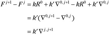
In all likelihood, the initial software development process and subsequent evolution processes will be materially different. This means that there will be a different proportionality constant, say k', representing the rate of fault introduction for the evolving system. For the total system, then, there will have been Fj = kR0 +k'∆0,j faults introduced into the system from the initial build through the jth build. Each module will have had ![]() faults introduced into it, either from the initial build or on subsequent builds. Thus, our revised estimate of the number of faults remaining in module i on build j will be:
faults introduced into it, either from the initial build or on subsequent builds. Thus, our revised estimate of the number of faults remaining in module i on build j will be:
![]()
The rate of fault introduction is directly related to the change activity that a module will receive from one build to the next. At the system level, we can see that the expected number of introduced faults from build j to build j+1 will be:
At the module level, the rate of fault introduction will again be proportional to the level of change activity. Hence, the expected number of introduced faults between build j to build j+1 on module i will be simply![]() .
.
The two proportionality constants k and k' are the ultimate criterion measures of the software development process and software maintenance processes. Each process has an associated fault introduction proportionality constant. If we institute a new software development process and observe a significant downward change in the constant k, then the change would have been a good one. Very frequently, however, software processes are changed because development fads change and not because a criterion measure has indicated that a new process is superior to a previous one. We will consider that an advance in software development process has occurred if either k or k' has diminished for that new process.
8.3.4 The Cassini System: A Case Study
To estimate rates of fault introduction, we now turn our attention to a complete software system on which every version of every module has been archived, together with the faults that have been recorded against the system as it evolved. [1], [2], [3], [4] On the first build of the Cassini system there were approximately 96K source lines of code in approximately 750 program modules. On the last build there were approximately 110K lines of source code in approximately 800 program modules. As the system progressed from the first to the last build, there were a total of 45,200 different versions of these modules. On the average, then, each module progressed through an average of 56 evolutionary steps or versions. For the purposes of this study, the Ada program module is a procedure or function. It is the smallest unit of the Ada language structure that can be measured. A number of modules present in the first build of the system were removed on subsequent builds. Similarly, a number of modules were added.
The Cassini Command and Data Subsytem (CDS) does not represent an extraordinary software system. It is quite typical of the amount of change activity that will occur in the development of a system on the order of 100 KLOC (thousand lines of code). It is a nontrivial measurement problem to track the system as it evolves. Again, there are two different sets of measurement activities that must occur at once. We are interested in both the changes in the source code and the fault reports that are being filed against each module.
To determine the efficiency of a test activity, it is necessary to have a system in which structural changes between one increment and its predecessor can be measured, together with the execution profile observed during test. Because we were unable to accomplish this for the Cassini CDS flight software, we studied the real-time software for a commercial embedded system. This will be discussed in Chapter 11.
In measuring the evolution of the system to talk about rates of fault introduction and removal, we measure in units proportional to the way the system changes over time. Changes to the system are visible at the module level, and we attempt to measure at that level of granularity. Because the measurements of system structure are collected at the module level (by module, we mean procedures and functions), information about faults must also be collected at the same granularity.
A fault, for the purposes of this particular investigation, is a structural imperfection in a software system that may lead to the system eventually failing. That is, it is a physical characteristic of the system of which the type and extent can be measured using the same ideas used to measure the properties of more traditional physical systems. Faults are introduced into a system by people making errors in their tasks. These errors can be errors of commission or errors of omission.
To count faults, there must be a well-defined method of identification that is repeatable, consistent, and identifies faults at the same level of granularity as our structural measurements. In analyzing the flight software for the Cassini Orbiter Command and Data Subsystem project at the Jet Propulsion Laboratory (JPL), the fault data and the source code change data were available from two different systems. The problem reporting information was obtained from the JPL institutional problem reporting system. For the Cassini system, failures were recorded starting at subsystem-level integration, and continuing through spacecraft integration and test. Failure reports typically contain descriptions of the failure at varying levels of detail, as well as descriptions of what was done to correct the fault(s) that caused the failure. Detailed information regarding the underlying faults (e.g., where were the code changes made in each affected module) is generally unavailable from the problem reporting system.
The entire source code evolution could be obtained directly from the Software Configuration Control System (SCCS) files for all versions of the flight software. The way in which SCCS was used in this development effort makes it possible to track changes to the system at a module level, in that each SCCS file stores the baseline version of that file (which may contain one or more modules) as well as the changes required to produce each subsequent increment (SCCS delta) of that file. When a module was created, or changed in response to a failure report or engineering change request, the file in which the module is contained was checked into SCCS as a new delta. This allowed us to track changes to the system at the module level as it evolved over time. For approximately 10 percent of the failure reports, we were able to identify the source file increment in which the fault(s) associated with a particular failure report were repaired. This information was available either in the comments inserted by the developer into the SCCS file as part of the check-in process, or as part of the set of comments at the beginning of a module that tracks its development history.
Using the information described above, we then set about to identify faults as per our working definition. For each problem report, the SCCS files were searched to identify all modules and the version(s) of each module for which the software was changed in response to the problem report. For each version of each module so identified, the assumption was made that all differences between the version in which repairs are implemented and the previous version are due solely to fault repair. This is not necessarily a valid assumption in that developers may also be making functional enhancements to the system in the same version that fault repairs are being made. Careful analysis of failure reports for which there was sufficiently detailed descriptive information served to separate areas of fault repair from other changes. A differential comparator (e.g., UNIX diff) was then used to obtain the differences between the versions in which the fault(s) were repaired and the immediately preceding version.
After completing the last step, the process of identifying and counting the faults began. The results of the differential comparison cannot simply be counted up to give a total number of faults. So that the faults could be reliably tallied, we developed a taxonomy for identifying and counting faults. [5] This taxonomy differs from others in that it does not seek to identify the root cause of the fault. Rather, it is based on the types of changes made to the software to repair the faults associated with failure reports. In other words, it constitutes an operational definition of a fault. We found that this taxonomy allowed us to identify faults in the software used in the study in a consistent manner at the appropriate level of granularity.
There was still substantial variability in the granularity of the definition of a fault. This was the primary motivation for the new definition for software faults shown in Chapter 5. Some of the faults in this study involved relatively little change in the code base. Other faults changed the code base materially. This granularity of measurement was simply not reflected in the taxonomy that we had developed for fault enumeration.
8.3.4.1 The Relationship between Faults and Code Changes.
Having established a theoretical relationship between software faults and code changes, it is now of interest to validate this model empirically. This measurement occurred on two simultaneous fronts. First, all versions of all the source code modules were measured. From these measurements, code churn and code deltas were obtained for every version of every module. The failure reports were sampled to lead to specific faults in the code. These faults were classified manually according to the above taxonomy and on a case-by-case basis. Then we were able to build a regression model relating the code measures to the code faults.
The Ada source code modules for all versions of each of these modules were systematically reconstructed from the SCCS code deltas. Each of these module versions was then measured by the UX-Metric analysis tool for Ada. Not all metrics provided by this tool were used in this study. Only a subset of these actually provide distinct sources of variation. The specific metrics used in this study are shown in Exhibit 21.
Exhibit 21: Software Metric Definitions
| Metrics | Definition |
|---|---|
| η1 | Count of unique operators |
| η2 | Count of unique operands |
| N1 | Count of total operators |
| N2 | Count of total operands |
| P/R | Purity ratio: ratio of Halstead's |
| V(g) | McCabe's cyclomatic complexity |
| Depth | Maximum nesting level of program blocks |
| AveDepth | Average nesting level of program blocks |
| LOC | Number of lines of code |
| Blk | Number of blank lines |
| Cmt | Count of comments |
| CmtWds | Total words used in all comments |
| Stmts | Count of executable statements |
| LSS | Number of logical source statements |
| PSS | Number of physical source statements |
| NonEx | Number of nonexecutable statements |
| AveSpan | Average number of lines of code between references to each variable |
| VI | Average variable name length |
To establish a baseline system, all of the metric data for the module versions that were members of the first build of CDS were then analyzed by our PCA-FI tool. This tool is designed to compute FI values, either from a baseline system or from a system being compared to the baseline system. In that the first build of the Cassini CDS system was selected to be the baseline system, the PCA-FI tool performed a principal components analysis on this data with an orthogonal varimax rotation. The objective of this phase of the analysis is to use the principal components technique to reduce the dimensionality of the metric set.
As can been seen in Exhibit 22, there are four principal components for the 18 metrics shown in Exhibit 20. For convenience, we have chosen to name these principal components as size, structure, style, and nesting. From the last row in Exhibit 22 we can see that the new reduced set of orthogonal components of the original 18 metrics account for approximately 85 percent of the variation in the original metric set.
Exhibit 22: Principal Components of Software Metrics
| Metric | Size | Structure | Style | Nesting |
|---|---|---|---|---|
| Stmts | 0.968 | 0.022 | -0.079 | 0.021 |
| LSS | 0.961 | 0.025 | -0.080 | 0.004 |
| N2 | 0.926 | 0.016 | 0.086 | 0.086 |
| N1 | 0.934 | 0.016 | 0.074 | 0.077 |
| η2 | 0.884 | 0.012 | -0.244 | 0.043 |
| AveSpan | 0.852 | 0.032 | 0.031 | -0.082 |
| V(g) | 0.843 | 0.032 | -0.094 | -0.114 |
| η1 | 0.635 | -0.055 | -0.522 | -0.136 |
| Depth | 0.617 | -0.022 | -0.337 | -0.379 |
| LOC | -0.027 | 0.979 | 0.136 | 0.015 |
| Cmt | -0.046 | 0.970 | 0.108 | 0.004 |
| PSS | -0.043 | 0.961 | 0.149 | 0.019 |
| CmtWds | 0.033 | 0.931 | 0.058 | -0.010 |
| NonEx | -0.053 | 0.928 | 0.076 | -0.009 |
| Blk | 0.263 | 0.898 | 0.048 | 0.005 |
| P/R | -0.148 | -0.198 | -0.878 | 0.052 |
| Vl | 0.372 | -0.232 | -0.752 | 0.010 |
| AveDepth | -0.000 | -0.009 | 0.041 | -0.938 |
| % Variance | 37.956 | 30.315 | 10.454 | 6.009 |
8.3.4.2 Estimation of the Proportionality Constant: An Example from Cassini.
As is fairly typical in the principal components analysis of metric data, the size domain dominates the analysis. It alone accounts for approximately 38 percent of the total variation in the original metric set. Not surprisingly, this domain contains the metrics of total statement count (Stmts), logical source statements (LSS), and the Halstead lexical metric primitives of operator and operand count, but it also contains cyclomatic complexity (V(g)). The structure domain contains those metrics relating to the physical structure of the program, such as nonexecutable statements (NonEx) and the program block count (Blk). The style domain contains measures of attribute that are directly under a programmer's control, such as variable length (Vl) and purity ratio (P/R). The nesting domain consists of the single metric that is a measure of the average depth of nesting of program modules (AveDepth).
To transform the raw metrics for each module version into their corresponding FI values, the means and the standard deviations must be computed. These are shown in Exhibit 23. These values will be used to transform all raw metric values for all versions of all modules to their baselined z-score values. The last four columns in Exhibit 23 contain the actual transformation matrix that will map the metric z-score values onto their orthogonal equivalents to obtain the orthogonal domain metric values used in the computation of FI. Finally, the eigenvalues for the four domains are presented in the last row of Exhibit 23.
Exhibit 23: Baseline Transformation Data for the Cassini Data
| Metric | | δB | Domain 1 | Domain 2 | Domain 3 | Domain 4 |
|---|---|---|---|---|---|---|
| Stmts | 11.37 | 7.79 | 0.10 | -0.02 | 0.26 | 0.05 |
| LSS | 25.18 | 27.08 | 0.13 | 0.00 | 0.04 | -0.09 |
| N2 | 79.59 | 129.08 | 0.13 | 0.02 | -0.17 | -0.08 |
| Nl | 68.24 | 115.72 | 0.13 | 0.02 | -0.17 | -0.09 |
| η2 | 1.32 | 0.54 | 0.00 | -0.07 | 0.54 | -0.16 |
| AveSpan | 4.77 | 6.19 | 0.12 | 0.01 | -0.03 | 0.07 |
| V(g) | 1.48 | 1.58 | 0.10 | -0.01 | 0.17 | 0.30 |
| η1 | 0.00 | 0.05 | 0.01 | 0.00 | 0.06 | 0.88 |
| Depth | 162.05 | 515.83 | -0.01 | 0.17 | 0.07 | -0.02 |
| LOC | 19.05 | 30.14 | 0.03 | 0.16 | 0.07 | -0.02 |
| Cmt | 34.19 | 124.24 | -0.01 | 0.17 | 0.09 | -0.01 |
| PSS | 139.27 | 452.48 | 0.00 | 0.16 | 0.10 | 0.00 |
| CmtWds | 16.61 | 20.44 | 0.14 | 0.01 | -0.07 | -0.05 |
| NonEx | 17.52 | 23.50 | 0.14 | 0.01 | -0.07 | -0.04 |
| Blk | 108.80 | 372.11 | -0.01 | 0.17 | 0.06 | -0.02 |
| P/R | 7.36 | 22.84 | -0.01 | 0.16 | 0.10 | 0.00 |
| V1 | 5.75 | 8.26 | 0.12 | 0.02 | -0.11 | 0.06 |
| AveDepth | 9.00 | 4.40 | 0.07 | -0.06 | 0.40 | -0.11 |
| Eigenvalues | 6.832 | 5.457 | 1.882 | 1.082 |
Exhibit 23, then, contains all of the essential information needed to obtain baselined FI values for any version of any module relative to the baseline build. As an aside, it is not necessary that the baseline build be the initial build. As a typical system progresses through hundreds of builds in the course of its life, it is well worth reestablishing a baseline closer to the current system. In any event, this baseline data is saved by the PCA-FI tool for use in later computation of metric values. Whenever the tool is invoked referencing the baseline data, it will automatically use this data to transform the raw metric values given to it.
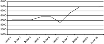
Exhibits 24 and 25 clearly show the evolution of the code across the ten builds of the system. By looking at the code deltas we can see that there was substantial change on build 4 to simplify the system. The total code delta went down. As we saw on the Space Shuttle PASS, this was immediately followed by a substantial upward swing in the code delta. Maximum change activity occurred between builds 3 and 7, as evidenced by the code churn values. The plot of system FI values in Exhibit 25 shows the typical net upward trend in total system complexity from the first build to the last.
Exhibit 24: Code Churn and Code Deltas across all Builds
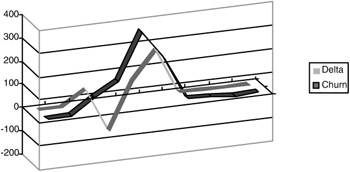
Exhibit 25: FI across all Builds
In relating the number of faults introduced in an increment to measures of a module's structural change, we had only a small number of observations with which to work. Problem reports could not be consistently traced back to source code. The net result was that of the more than 100 faults that were initially identified, there were only 35 observations in which a fault could be associated with a particular increment of a module, and with that increment's measures of code delta and code churn.
For each of the 35 modules for which there was viable fault data, there were three data points. First, we had the number of introduced faults for that module that were the direct result of changes that had occurred on that module between the current version that contained the faults and the previous version that did not. Second, we had code delta values for each of these modules from the current to the previous version. Finally, we had code churn values derived from the code deltas.
Linear regression models were formulated for code churn and code deltas with code faults as the dependent variable in both cases. Both models were built without constant terms in that we surmise that if no changes were made to a module, then no new faults could be introduced. The results of the regression between faults and code deltas were not at all surprising. The squared multiple R for this model was 0.001, about as close to zero as you can get. This result is directly attributable to the nonlinearity of the data. Change comes in two flavors: change can increase the complexity of a module or change can decrease the complexity of a model. Faults, on the other hand, are not related to the direction of the change but to its intensity. Removing masses of code from a module is just as likely to introduce faults as adding code to it.
The regression model between code churn and faults is dramatically different. The regression ANOVA for this model is shown in Exhibit 26. Whereas code deltas do not show a linear relationship with faults, code churn certainly does. The actual regression model is given in Exhibit 27. The regressions statistics are summarized in Exhibit 28. Of particular interest in Exhibit 28 is the Squared Multiple R term. This has a value of 0.649. This means, roughly, that the regression model will account for more than 65 percent of the variation in the faults of the observed modules based on the values of code churn.
Exhibit 26: Regression Analysis of Variance
| Source | Sum of Squares | DF | Mean Square | F Ratio | P |
|---|---|---|---|---|---|
| Regression | 331.879 | 1 | 331.879 | 62.996 | 0.00 |
| Residual | 179.121 | 34 | 10.673 | 5.268 |
Exhibit 27: Regression Model
| Effect | Coefficient | Std. Error | t | P(2-Tail) |
|---|---|---|---|---|
| Churn | 0.576 | 0.073 | 7.937 | 0.000 |
Exhibit 28: Regression Statistics
| N | Multiple R | Squared Multiple R | Standard Error of Estimate |
|---|---|---|---|
| 35 | 0.806 | 0.649 | 2.296 |
The regression coefficient shown in Exhibit 27 is, in fact, the estimate of the proportionality constant k'. This is the relative rate of fault introduction as a function of code churn.
[1]Munson, J.C., Software Faults, Software Failures, and Software Reliability Modeling, Information and Software Technology, December 1996.
[2]Nikora, A.P., Software System Defect Content Prediction from Development Process and Product Characteristics, Doctoral dissertation, Department of Computer Science, University of Southern California, Los Angeles, May 1998.
[3]Nikora, A.P. and Munson, J.C., Software Evolution and the Fault Process, Proceedings of the 23rd Annual Software Engineering Workshop, NASA/Goddard Space Flight Center (GSFC) Software Engineering Laboratory (SEL), Greenbelt, MD, 1998.
[4]Nikora, A.P. and Munson, J.C., Determining Fault Insertion Rates for Evolving Software Systems, Proceedings of the 1998 IEEE International Symposium of Software Reliability Engineering, Paderborn, Germany, November 1998, IEEE Computer Society Press.
[5]Nikora, A.P. and Munson, J.C., Determining Fault Insertion Rates for Evolving Software Systems, Proceedings of the 1998 IEEE International Symposium of Software Reliability Engineering, Paderborn, Germany, November 1998, IEEE Computer Society Press.
|
|
EAN: 2147483647
Pages: 139
- The Second Wave ERP Market: An Australian Viewpoint
- Context Management of ERP Processes in Virtual Communities
- Distributed Data Warehouse for Geo-spatial Services
- A Hybrid Clustering Technique to Improve Patient Data Quality
- Relevance and Micro-Relevance for the Professional as Determinants of IT-Diffusion and IT-Use in Healthcare
- Chapter II Information Search on the Internet: A Causal Model
- Chapter III Two Models of Online Patronage: Why Do Consumers Shop on the Internet?
- Chapter IV How Consumers Think About Interactive Aspects of Web Advertising
- Chapter XVII Internet Markets and E-Loyalty
- Chapter XVIII Web Systems Design, Litigation, and Online Consumer Behavior