Structured Query Language (SQL)
| Structured Query Language (SQL) is a standardized language used to work with database objects and the data they contain. Using SQL, you can define, alter, and remove database objects, as well as add, update, delete, and retrieve data values. One of the strengths of SQL is that it can be used in a variety of ways: SQL statements can be executed interactively using tools such as the Command Center and the Command Line Processor, they can be placed directly in UNIX shell scripts or Windows batch files, and they can be embedded in high-level programming language source code files that are precompiled/compiled to create a database application. (Because SQL is nonprocedural by design, it is not an actual programming language; therefore, most embedded SQL applications are built by combining the decision and sequence control of a high-level programming language with the data storage, manipulation, and retrieval capabilities of SQL). Like most other languages, SQL has a defined syntax and a set of language elements. Most SQL statements can be categorized according to the function they have been designed to perform; SQL statements typically fall under one of the following categories:
You do not have to be familiar with the Embedded SQL Application Construct Statements in order to pass the DB2 UDB V8.1 Family Fundamentals certification exam (Exam 700). However, you must know how the more common DCL, DDL, and DML statements are used, and you must be familiar with the Transaction Management Statements available. With that in mind, this chapter will focus on introducing you to the most common SQL statements used to create database objects and manipulate data.
Data Control Language (DCL) StatementsYou may recall that in Chapter 3, "Security," we saw that authorities and privileges are used to control access to the DB2 Database Manager for an instance, to one or more databases running under that instance's control, and to a particular database's objects. Users are only allowed to work with those objects for which they have been given the appropriate authority or privilege; the authorities and privileges they possess also determine what they can and cannot do with the objects they have access to. Authorities and privileges are given using the GRANT SQL statement. Likewise, authorities and privileges are revoked using the REVOKE SQL statement. The GRANT statement and the REVOKE statement, along with the CONNECT SQL statement, make up the bulk of the Data Control Language (DCL) statements available with DB2 UDB. The CONNECT statementBefore a user can access data stored in a DB2 UDB database (or do anything else with a database for that matter), they must first establish a connection to that database. In some cases, a database connection can be established using the Control Center; however, in most cases, a database connection is established by executing the CONNECT SQL statement. The basic syntax for this statement is: CONNECT TO [ DatabaseName ] <USER [ UserID ] USING [ Password ]> where:
Thus, in order for a user whose authentication ID is "db2user" and whose password is "ibmdb2" to establish a connection to a database named SAMPLE, a CONNECT statement that looks something like this would need to be executed: CONNECT TO SAMPLE USER db2user USING ibmdb2 And as soon as the CONNECT statement is successfully executed, you might see a message that looks something like this: Database Connection Information Database server = DB2/NT 8 SQL authorization ID = DB2USER Local database alias = SAMPLE
Once a database connection has been established, it will remain in effect until it is explicitly terminated or until the application that established the connection ends. Database connections can be explicitly terminated at any time by executing a special form of the CONNECT statement. The syntax for this form of the CONNECT statement is: CONNECT RESET The GRANT statement (revisited)In Chapter 3, "Security," we saw that authorities and privileges can be explicitly granted to an individual user or a group of users by executing the GRANT SQL statement. Several flavors of the GRANT statement are available, and the appropriate form to use is determined by the database object for which authorities and privileges are to be granted. (Objects for which authorities and privileges can be granted include databases, schemas, tablespaces, tables, indexes, views, packages, routines, sequences, servers, and nicknames.) In general, the basic syntax for the GRANT statement looks something like this: GRANT [Privilege] ON [ObjectType] [ObjectName] TO [ Recipient , ...] <WITH GRANT OPTION> where:
If the WITH GRANT OPTION clause is specified with the GRANT statement, the user and/or group receiving the specified privileges is given the ability to grant the newly received privileges (except for the CONTROL privilege) to other users. For more information about available authorities and privileges, and for examples of how the GRANT SQL statement can be used, refer to Chapter 3, "Security." The REVOKE statement (revisited)Authorities and privileges can be explicitly revoked from an individual user or a group of users by executing the REVOKE SQL statement. As with the GRANT SQL statement, several flavors of the REVOKE statement are available, and the appropriate form to use is determined by the database object for which authorities and privileges are to be revoked. In general, the basic syntax for the REVOKE statement looks something like this: REVOKE [Privilege] ON [ObjectType] [ObjectName] FROM [ Forfeiter , ...] <BY ALL> where:
The BY ALL clause is optional and is provided as a courtesy for administrators who are familiar with the syntax of the DB2 for OS/390 REVOKE SQL statement. Whether it is included or not, the results will always be the same ”the privilege(s) specified will be revoked from all users and/or groups specified, regardless of who granted it originally. Again, for more information about the authorities and privileges available, and for examples of how the REVOKE statement can be used, refer to Chapter 3, "Security." Data Definition Language (DDL) StatementsWhen a database is first created, it cannot be used to store data because, aside from the read-only system catalog tables and views that get created by default, no other data objects exist. That's where the Data Definition Language (DDL) statements come into play. The Data Definition Language statements are a set of SQL statements that are used to define and create objects in a database that will be used both to store user data and to improve data access performance. Various forms of CREATE statements and ALTER statements, along with the DROP statement, make up the set of Data Definition Language (DDL) statements available with DB2 UDB. The CREATE BUFFERPOOL statementEarlier, we saw that a buffer pool is an area of main memory that has been allocated to the DB2 Database Manager for the purpose of caching table and index data pages as they are read from disk. By default, one buffer pool (named IBMDEFAULTBP) is created for a particular database when that database is first created. On Linux and UNIX platforms, this buffer pool is 1,000 4K (kilobyte) pages in size; on Windows platforms, this buffer pool is 250 4K pages in size. Additional buffer pools can be created by executing the CREATE BUFFERPOOL SQL statement. The basic syntax for this statement is: CREATE BUFFERPOOL [ BufferPoolName ] <IMMEDIATE DEFERRED> SIZE [ Size ] <PAGESIZE [ PageSize ] <K>> <NOT EXTENDED STORAGE EXTENDED STORAGE> where:
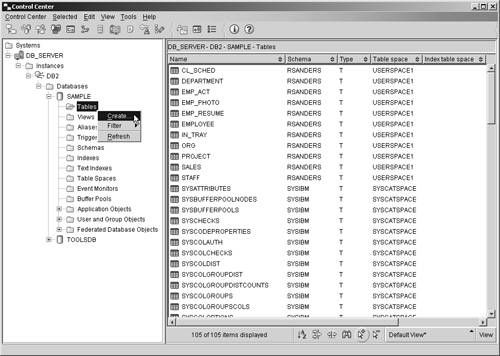
If the IMMEDIATE clause is specified with the CREATE BUFFERPOOL statement, the buffer pool will be created immediately unless the amount of memory required is not available, in which case a warning message will be generated and the buffer pool creation process will behave as if the DEFERRED clause were specified. If the DEFERRED clause is specified, the buffer pool will not be created until all connections to the database the buffer pool is to be created for have been terminated. If neither clause is specified, the buffer pool will not be created until all connections to the database the buffer pool is to be created for have been terminated. So, if you wanted to create a buffer pool that has the name TEMP_BP, consists of 100 pages that are 8 kilobytes in size, and is to be created immediately if enough free memory is available, you could do so by executing a CREATE BUFFERPOOL SQL statement that looks something like this: CREATE BUFFERPOOL TEMP_BP IMMEDIATE SIZE 100 PAGESIZE 8 K Buffer pools can also be created using the Create Buffer Pool dialog, which can be activated by selecting the appropriate action from the Buffer Pools menu found in the Control Center. Figure 5-1 shows the Control Center menu items that must be selected to activate the Create Buffer Pool dialog; Figure 5-2 shows how the Create Buffer Pool dialog might look after its input fields have been populated . Figure 5-1. Invoking the Create Buffer Pool dialog from the Control Center. Figure 5-2. The Create Buffer Pool dialog. The CREATE TABLESPACE statementAs mentioned earlier, tablespaces are used to control where data is physically stored and to provide a layer of indirection between database objects and the directories, files, or raw devices (referred to as containers) in which the data physically resides. Depending upon how it is defined, a tablespace can be either a System Managed Space (SMS) tablespace or a Database Managed Space (DMS) tablespace. With SMS tablespaces, each container used must be a directory that resides within the file space of the operating system, and the operating system's file manager is responsible for managing data storage. With DMS tablespaces, each container used must be either a fixed-size preallocated file or a raw device, and the DB2 Database Manager is responsible for managing data storage. By default, three tablespaces (named SYSCATSPACE, USERSPACE1, and TEMPSPACE1) are created for a database as part of the database creation process. Additional tablespaces can be created by executing the CREATE TABLESPACE SQL statement. The basic syntax for this statement is: [View full width]
or [View full width]
where:
If the MANAGED BY SYSTEM version of this statement is executed, the resulting tablespace will be an SMS tablespace. On the other hand, if the MANAGED BY DATABASE version is executed, the resulting tablespace will be a DMS tablespace. Furthermore, if an SMS tablespace is to be created, only existing directories can be used as that tablespace's storage container(s), and if a DMS tablespace is to be created, only fixed-size preallocated files or physical raw devices can be used as that tablespace's storage container(s).
Thus, if you wanted to create a DMS tablespace that has the name PAYROLL_TS, consists of pages that are 8 kilobytes in size, uses the file DMS_TBS, which is 1000 megabytes in size and resides in the directory C:\TABLESPACES as its storage container, and uses the buffer pool PAYROLL_BP, you could do so by executing a CREATE TABLESPACE SQL statement that looks something like this: CREATE TABLESPACE PAYROLL_TS PAGESIZE 8K MANAGED BY DATABASE USING (FILE 'C:\TABLESPACES\DMS_TBSP.TSF', 100 M) BUFFERPOOL PAYROLL_BP Tablespaces can also be created using the Create Table Space Wizard, which can be activated by selecting the appropriate action from the Table Spaces menu found in the Control Center. Figure 5-3 shows the Control Center menu items that must be selected to activate the Create Table Space Wizard; Figure 5-4 shows how the first page of the Create Table Space Wizard might look after its input fields have been populated. Figure 5-3. Invoking the Create Table Space Wizard from the Control Center. Figure 5-4. The first page of the Create Table Space Wizard. The ALTER TABLESPACE statementBecause SMS tablespaces rely on the operating system for physical storage space management, they rarely need to be modified after they have been successfully created. DMS tablespaces, on the other hand, have to be monitored closely to ensure that the fixed-size preallocated file(s) or physical raw device(s) that they use for storage always have enough free space available to meet the database's needs. When the amount of free storage space available to a DMS tablespace becomes dangerously low (typically less than 10 percent), more free space can be added either by increasing the size of one or more of its containers or by making one or more new containers available to it. Existing tablespace containers can be resized, new containers can be made available to an existing tablespace, and an existing tablespace's properties can be altered by executing the ALTER TABLESPACE SQL statement. The basic syntax for this statement is: ALTER TABLESPACE [ TablespaceName ] ADD ( [FILE DEVICE] '[ Container ]' [ ContainerSize ] ,... ) or ALTER TABLESPACE [ TablespaceName ] DROP ( [FILE DEVICE] '[ Container ]' ,... ) or ALTER TABLESPACE [ TablespaceName ] [EXTEND REDUCE RESIZE] ( [FILE DEVICE] '[ Container ]' ,... ) or ALTER TABLESPACE [ TablespaceName ] <PREFETCHSIZE [ PrefetchPages PrefetchSize <K M G>]> <BUFFERPOOL [ BufferPoolName ]> <DROPPED TABLE RECOVERY [ON OFF]> where:
Thus, if you wanted a fixed-size preallocated file named NEWFILE.TSF, which is 1000 megabytes in size and resides in the directory C:\TABLESPACES, to be used as a new storage container for an existing DMS tablespace named PAYROLL_TS, you could make the PAYROLL_TS tablespace use this file as a new storage container by executing an ALTER TABLESPACE SQL statement that looks like this: ALTER TABLESPACE PAYROLL_TS ADD (FILE 'C:\TABLESPACES\NEWFILE.TSF', 100 M) Tablespaces can also be altered using the Alter Table Space dialog, which can be activated by selecting the appropriate action from the Table Spaces menu found in the Control Center. Figure 5-5 shows the Control Center menu items that must be selected in order to activate the Alter Table Space dialog; Figure 5-6 shows how the first page of the Alter Table Space dialog might look after its input fields have been populated. Figure 5-5. Invoking the Alter Table Space dialog from the Control Center. Figure 5-6. The first page of the Alter Table Space dialog. The CREATE TABLE statementEarlier, we saw that a table is a logical structure used to present data as a collection of unordered rows with a fixed number of columns . Each column contains a set of values of the same data type, and each row contains the actual table data. Because tables are the basic data objects used to store information, many are often created for a single database. Tables are created by executing the CREATE TABLE SQL statement. In its simplest form, the syntax for this statement is: CREATE TABLE [ TableName ] ([ColumnName] [DataType] ,...) where:
Table 5-1. Data Type Definitions That Can Be Used with the CREATE TABLE Statement
Thus, if you wanted to create a table that had three columns in it, two of which are used to store numeric values and one that is used to store character string values, you could do so by executing a CREATE TABLE SQL statement that looks something like this: CREATE TABLE EMPLOYEES (EMPID INTEGER, NAME CHAR(50), DEPT INTEGER) It is important to note that this is an example of a relatively simple table. Table definitions can be quite complex, and as a result, the CREATE TABLE statement has several different permutations . Because the definition for a table object can be so complex, and because the syntax for the CREATE TABLE SQL statement can be complex as well, both are covered in much more detail in Chapter 6, "Working With DB2 UDB Objects." (A detailed description of available data types is presented in Chapter 6 as well.) Like many of the other database objects available, tables can be created using a GUI tool that is accessible from the Control Center. In this case, the tool is the Create Table Wizard, and it can be activated by selecting the appropriate action from the Tables menu found in the Control Center. Figure 5-7 shows the Control Center menu items that must be selected to activate the Create Table Wizard; Figure 5-8 shows how the first page of the Create Table Wizard might look after its input fields have been populated. Figure 5-7. Invoking the Create Table Wizard from the Control Center. Figure 5-8. The first page of the Create Table Wizard. The ALTER TABLE statementOver time, a table may be required to hold additional data values that did not exist or were not considered at the time the table was created. Or character data that was originally thought to be one size may have turned out to be larger than was anticipated. These are just a couple of reasons why it can become necessary to modify an existing table's definition. When the amount of data stored in a table is relatively small, and when the table has few or no dependencies, it is relatively easy to save the associated data, drop the existing table, create a new table incorporating the appropriate modifications, load the previously saved data into the new table, and redefine all appropriate dependencies. But how can you make such modifications to a table that holds a large volume of data or has numerous dependency relationships? Certain properties of an existing table can be changed, additional columns and constraints can be added (constraints are covered in detail in Chapter 6, "Working with DB2 UDB Objects"), existing constraints can be removed, and the length of varying-length character data type values allowed for a particular column can be increased by executing the ALTER TABLE SQL statement. Like the CREATE TABLE statement, the ALTER TABLE statement can be quite complex. However, in its simplest form, the syntax for the ALTER TABLE statement is: ALTER TABLE [ TableName ] ADD [ Element ,...] or ALTER TABLE [ TableName ] ALTER COLUMN [ ColumnName ] SET DATA TYPE [VARCHAR CHARACTER VARYING CHAR VARYING] ([ Length ]) or ALTER TABLE [ TableName ] DROP [PRIMARY KEY FOREIGN KEY [ ConstraintName ] UNIQUE [ ConstraintName ] CHECK [ ConstraintName ] CONSTRAINT [ ConstraintName ]] where:
The basic syntax used to add a new column is: <COLUMN> [ColumnName] [DataType] <NOT NULL WITH DEFAULT <[ DefaultValue ] CURRENT DATE CURRENT TIME CURRENT TIMESTAMP>> < UniqueConstraint > < CheckConstraint > < ReferentialConstraint > where:
The ALTER TABLE statement syntax used to add a unique or primary key constraint, a check constraint, and/or a referential constraint as part of a column definition is the same as the syntax used with the more advanced form of the CREATE TABLE statement. This syntax, along with details on how each of these constraints is used, is covered in Chapter 6, "Working with DB2 UDB Objects." So if you wanted to add two new columns that use a date data type to an existing table named EMPLOYEES, you could do so by executing an ALTER TABLE SQL statement that looks something like this: ALTER TABLE EMPLOYEES ADD COLUMN BIRTHDAY DATE ADD COLUMN HIREDATE DATE On the other hand, if you wanted to change the maximum length of the data value allowed for a varying-length character data type column named DEPTNAME found in a table named DEPARTMENT from 50 to 100, you could do so by executing an ALTER TABLE statement that looks something like this: ALTER TABLE DEPARTMENT ALTER COLUMN DEPTNAME SET DATA TYPE VARCHAR(100) As you might imagine, existing tables can also be modified using the Alter Table dialog, which can be activated by selecting the appropriate action from the Tables menu found in the Control Center. Figure 5-9 shows the Control Center menu items that must be selected in order to activate the Alter Table dialog; Figure 5-10 shows how the Alter Table dialog might look after its input fields have been populated. Figure 5-9. Invoking the Alter Table dialog from the Control Center. Figure 5-10. The Alter Table dialog. The CREATE INDEX statementIt was mentioned earlier that an index is an object that contains an ordered set of pointers that refer to records stored in a base table. Indexes are important because they:
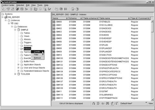
While some indexes are created implicitly to provide support for a table's definition (for example to provide support for a primary key), indexes are typically created explicitly, using the tools provided with DB2 UDB. Indexes can be created by executing the CREATE INDEX SQL statement. The basic syntax for this statement is: CREATE <UNIQUE> INDEX [ IndexName ] ON [ TableName ] ( [ PriColumnName ] <ASC DESC> ,... ) <INCLUDE ( [ SecColumnName ] ,... )> <CLUSTER> <DISALLOW REVERSE SCANS ALLOW REVERSE SCANS> where:
If the UNIQUE clause is specified when the CREATE INDEX statement is executed, rows in the table associated with the index to be created must not have two or more occurrences of the same values in the set of columns that make up the index key. If the base table the index is to be created for contains data, this uniqueness is checked when the DB2 Database Manager attempts to create the index specified; once the index has been created, this uniqueness is enforced each time an insert or update operation is performed against the table. In both cases, if the uniqueness of the index key is compromised, the index creation, insert, or update operation will fail, and an error will be generated. It is important to keep in mind that when the UNIQUE clause is used, it is possible to have an index key that contains one (and only one) NULL value. So, if you wanted to create a unique index for a base table named EMPLOYEES that has the following characteristics:
such that the index key consists of the column named EMPNO, you could do so by executing a CREATE INDEX statement that looks something like this: CREATE INDEX EMPNO_INDX ON EMPLOYEES (EMPNO) Indexes can also be created using the Create Index dialog, which can be activated by selecting the appropriate action from the Indexes menu found in the Control Center. Figure 5-11 shows the Control Center menu items that must be selected to activate the Create Indexes dialog; Figure 5-12 shows how the Create Indexes dialog might look after its input fields have been populated. Figure 5-11. Invoking the Create Index dialog from the Control Center. Figure 5-12. The Create Index dialog. If an index is created for an empty table, that index will not have any entries stored in it until the table the index is associated with is populated. On the other hand, if an index is created for a table that already contains data, index entries will be generated for the existing data and added to the index as soon as it is created. Any number of indexes can be created for a table, using a wide variety of combinations of columns. However each index comes at a price in both storage requirements and performance: Since each index replicates its key values, and this replication requires additional storage space, and each modification to a table results in a similar modification to all indexes defined on the table, performance can decrease when insert, update, and delete operations are performed. In fact, if a large number of indexes are created for a table that is modified frequently, overall performance will decrease, rather than increase for all operations except data retrieval. Tables that are used for data mining, business intelligence, business warehousing, and other applications that execute many (and often complex) queries while rarely modifying data are prime targets for multiple indexes. On the other hand, tables that are used in OLTP (On-Line Transactional Processing) environments or other environments where data throughput is high should use indexes sparingly. The CREATE VIEW statementWe saw earlier that a view is an object that acts as a named specification of a result data set that is produced each time the view is referenced. A view can be thought of as having columns and rows, just like base tables, and in most cases, data can be retrieved directly from a view in the same way that it can be retrieved from a base table. However, whether a view can be used to insert, update, or delete data depends on how it is defined. (In general, a view can be used in an insert, update, or delete operation if each row in the view can be uniquely mapped onto a single row of a base table.) Although views look (and often behave) like base tables, they do not have their own physical storage (contrary to indexes, which are also based on base tables); therefore, they do not contain data. Instead, views refer to data that is physically stored in other base tables. And because a view can reference the data stored in any number of columns found in the base table it refers to, views can be used, together with view privileges, to control what data a user can and cannot see. For example, suppose a company has a database that contains a table that has been populated with information about each employee of that company. Managers might work with a view that only allow them to see information about employees they manage, while users in Corporate Communications might work with a view that only allows them to see contact information about each employee, and users in Payroll might work with a view that allows them to see both contact information and salary information. By creating views and coupling them with the view privileges available, a database administrator can have greater control over how individual users access specific pieces of data. Views can be created by executing the CREATE VIEW SQL statement. The basic syntax for this statement is: CREATE VIEW [ ViewName ] <( [ ColumnName ] ,... )> AS [ SELECTStatement ] <WITH CHECK OPTION> where:
Thus, if you wanted to create a view that references all data stored in a table named DEPARTMENT and assign it the name DEPT_VIEW, you could do so by executing a CREATE VIEW SQL statement that looks something like this: CREATE VIEW DEPT_VIEW AS SELECT * FROM DEPARTMENT On the other hand, if you wanted to create a view that references specific data values stored in the table named DEPARTMENT and assign it the name ADV_DEPT_VIEW, you could do so by executing a CREATE VIEW SQL statement that looks something like this: CREATE VIEW ADV_DEPT_VIEW AS SELECT (DEPT_NO, DEPT_NAME, DEPT_SIZE) FROM DEPARTMENT WHERE DEPT_SIZE > 25 The view created by this statement would only contain department number, department name, and department size information for each department that has more than 25 people in it. Views can also be created using the Create View dialog, which can be activated by selecting the appropriate action from the Views menu found in the Control Center. Figure 5-13 shows the Control Center menu items that must be selected to activate the Create View dialog; Figure 5-14 shows how the Create View dialog might look after its input fields have been populated. Figure 5-13. Invoking the Create View dialog from the Control Center. Figure 5-14. The Create View dialog. If the WITH CHECK OPTION clause of with the CREATE VIEW SQL statement is specified, insert and update operations performed against the view that is created are validated to ensure that all rows being inserted into or updated in the base table the view refers to conform to the view's definition (otherwise, the insert/update operation will fail). So what exactly does this mean? Suppose a view was created using the following CREATE VIEW statement: CREATE VIEW PRIORITY_ORDERS AS SELECT * FROM ORDERS WHERE RESPONSE_TIME < 4 WITH CHECK OPTION Now, suppose a user tries to insert a record into this view that has a RESPONSE_TIME value of 6. The insert operation will fail because the record violates the view's definition. Had the view not been created with the WITH CHECK OPTION clause, the insert operation would have been successful, even though the new record would not be visible to the view that was used to add it. Figure 5-15 illustrates how the WITH CHECK OPTION works. Figure 5-15. How the WITH CHECK OPTION clause is used to ensure insert and update operations conform to a view's definition.
The CREATE ALIAS statementWe saw earlier that an alias is simply an alternate name for a table or view and that once created, aliases can be referenced the same way tables or views can be referenced. By using aliases, SQL statements can be constructed such that they are independent of the qualified names that identify the base tables or views they reference. Whenever an alias is used in an SQL statement, the behavior is the same as when the target (source table or view) of the alias is used instead. Therefore, any application that uses an alias to access data can easily be made to work with many different targets. That's because when the target of an alias is changed, no changes to applications that use the alias are necessary. Aliases can be created by executing the CREATE ALIAS SQL statement. The basic syntax for this statement is: CREATE [ALIAS SYNONYM] [ AliasName ] FOR [ TableName ViewName ExistingAlias ] where:
Thus, if you wanted to create an alias that references a table named EMPLOYEES and you wanted to assign it the name EMPINFO, you could do so by executing a CREATE ALIAS SQL statement that looks something like this: CREATE ALIAS EMPINFO FOR EMPLOYEES Aliases can also be created using the Create Alias dialog, which can be activated by selecting the appropriate action from the Alias menu found in the Control Center. Figure 5-16 shows the Control Center menu items that must be selected to activate the Create Alias dialog; Figure 5-17 shows how the Create Alias dialog might look after its input fields have been populated. Figure 5-16. Invoking the Create Alias dialog from the Control Center. Figure 5-17. The Create Alias dialog. The CREATE SCHEMA statementEarlier, we saw that a schema is an identifier that helps provide a means of classifying or grouping objects stored in a database. And because a schema is an object itself, it can be owned by an individual, who can control access to both the data and the objects that reside within it. Whenever a data object, such as a table, view, or index, is created, it is always assigned, either implicitly or explicitly, to a schema. Schemas are implicitly created whenever a data object that has been assigned a qualifier name that is different from existing schema names found in the database is created ”provided the user creating the object holds IMPLICIT_SCHEMA authority. (If a qualifier is not included as part of the name assigned to an object during the creation process, the authorization ID of the user creating the object is used as the schema, by default.) Schemas can be explicitly created by executing the CREATE SCHEMA SQL statement. The basic syntax for this statement is: CREATE SCHEMA [ SchemaName ] < SQLStatement ,...> or CREATE SCHEMA AUTHORIZATION [ AuthorizationName ] < SQLStatement ,...> or CREATE SCHEMA [ SchemaName ] AUTHORIZATION [ AuthorizationName ] < SQLStatement ,...> where:
If a schema name is specified, but no authorization name is provided, the authorization ID of the user that issued the CREATE SCHEMA statement is given ownership of the new schema when it is created; if an authorization name is specified but no schema name is provided, the new schema is assigned the same name as the authorization name used. So, if you wanted to explicitly create a schema named INVENTORY, along with a table named PARTS that is associated with the schema named INVENTORY, you could do so by executing a CREATE SCHEMA SQL statement that looks something like this: CREATE SCHEMA INVENTORY CREATE TABLE PARTS (PARTNO INTEGER NOT NULL, DESCRIPTION VARCHAR(50), QUANTITY SMALLINT) Schemas can also be created using the Create Schema dialog, which can be activated by selecting the appropriate action from the Schemas menu found in the Control Center. Figure 5-18 shows the Control Center menu items that must be selected to activate the Create Schema dialog; Figure 5-19 shows how the Create Schema dialog might look after its input fields have been populated. Figure 5-18. Invoking the Create Schema dialog from the Control Center. Figure 5-19. The Create Schema dialog. Since schemas can be implicitly created by creating an object with a new schema name, you may be wondering why anyone would want to explicitly create a schema using the CREATE SCHEMA statement or the Create Schema dialog. The primary reason for explicitly creating a schema has to do with access control. An explicitly created schema has an owner, identified either by the authorization ID of the user who executed the CREATE SCHEMA statement or by the authorization ID provided to identify the owner when the schema was created. A schema owner has the authority to create, alter, and drop any object stored in the schema; to drop the schema itself; and to grant these privileges to other users. On the other hand, implicitly created schemas are considered to be owned by the user "SYSIBM." Any user can create an object in an implicitly created schema, and each object in the schema is controlled by the user who created it. Furthermore, only users with System Administrator (SYSADM) or Database Administrator (DBADM) authority are allowed to drop implicitly created schemas. Thus, in order for a user other than a system administrator or database administrator to have complete control over a schema, as well as all data objects stored in it, the schema must be created explicitly. The CREATE TRIGGER statementWe saw earlier that a trigger is a group of actions that are automatically executed (or "triggered") whenever an insert, update, or delete operation is performed against a particular table. Triggers are often used in conjunction with constraints to enforce data integrity rules. However, triggers can also be used to automatically perform operations on other tables, to automatically generate and/or transform values for new or existing rows, to generate audit trails, and to detect exception conditions. By using triggers, the logic needed to enforce business rules can be placed directly in the database instead of in one or more applications; and by requiring the database to enforce business rules, the need to recode and recompile database applications each time business rules change is eliminated. Before a trigger can be created, the following components must be identified:
Triggered actions can refer to the values in the set of affected rows using what are known as transition variables. Transition variables use the names of the columns in the subject table, qualified by a specified name that indicates whether the reference is to the original value (before the insert, update, or delete operation is performed) or the new value (after the insert, update, or delete operation is performed). Another means of referring to values in the set of affected rows is through the use of transition tables. Transition tables also use the names of the columns in the subject table, but they allow the complete set of affected rows to be treated as a table. Unfortunately, transition tables can only be used in after triggers. Once the appropriate trigger components have been identified, a trigger can be created by executing the CREATE TRIGGER SQL statement. The basic syntax for this statement is: CREATE TRIGGER [ TriggerName ] [NO CASCADE BEFORE AFTER] [INSERT DELETE UPDATE <OF [ ColumnName ], ... >] ON [ TableName ] <REFERENCING [ Reference ]> [FOR EACH ROW FOR EACH STATEMENT] MODE DB2SQL <WHEN ( [ SearchCondition ] )> [ TriggeredAction ] where:
<OLD <AS> [ CorrelationName ]> <NEW <AS> [ CorrelationName ]> <OLD TABLE <AS> [ Identifier ]> <NEW TABLE <AS> [ Identifier ]> where:
Thus, if you wanted to create a trigger for a base table named EMPLOYEES that has the following characteristics:
that will cause the value for the column named EMPNO to be incremented each time a row is added to the table, you could do so by executing a CREATE TRIGGER statement that looks something like this: CREATE TRIGGER EMPNO_INC AFTER INSERT ON EMPLOYEES FOR EACH ROW MODE DB2SQL UPDATE EMPNO SET EMPNO = EMPNO + 1 Triggers can also be created using the Create Trigger dialog, which can be activated by selecting the appropriate action from the Triggers menu found in the Control Center. Figure 5-20 shows the Control Center menu items that must be selected to activate the Create Trigger dialog; Figure 5-21 shows how the Create Trigger dialog might look after its input fields have been populated. Figure 5-20. Invoking the Create Trigger dialog from the Control Center. Figure 5-21. The Create Trigger dialog. The DROP statementJust as it is important to be able to create and modify objects, it is important to be able to delete an existing object when it is no longer needed. Existing objects can be removed from a database by executing the DROP SQL statement. The basic syntax for this statement is: DROP [ ObjectType ] [ ObjectName ] where:
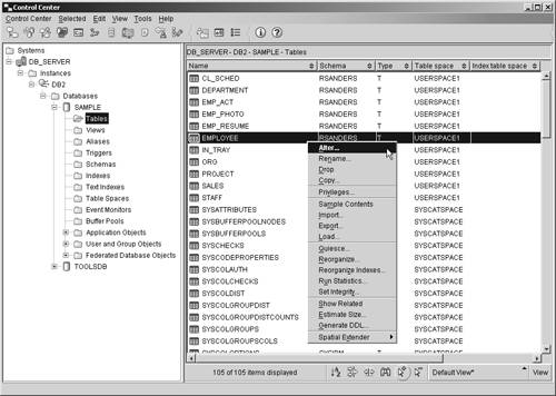
So, if you wanted to delete a table that has been assigned the name SALES, you could do so by executing a DROP SQL statement that looks something like this: DROP TABLE SALES Database objects can also be dropped from the Control Center by highlighting the appropriate object and selecting the appropriate action from any object menu found. Figure 5-22 shows the Control Center menu items that must be selected in order to drop a particular object (in this case, a tablespace object). Figure 5-22. Dropping a tablespace object from the Control Center. It is important to keep in mind that when an object is dropped, its removal may affect other objects that depend upon its existence. In some cases, when an object is dropped, all objects dependent upon that object are dropped as well (for example, if a tablespace containing one or more tables is dropped, all tables that resided in that tablespace, along with their corresponding data, are also dropped). In other cases, an object cannot be dropped if other objects are dependent upon its existence (for example, a schema can only be dropped after all objects that were in that schema have been dropped). And it goes without saying that built-in objects, such as the system catalog tables and views, cannot be dropped.
Data Manipulation Language (DML) StatementsOnce the appropriate data objects have been created for a particular database, they can be used to store data values. And just as there is a set of SQL statements that is used to define and create objects, there is a set of SQL statements that is used exclusively to store, modify, remove, and retrieve data values. This set of statements is referred to as Data Manipulation Language (DML) statements. There are four Data Manipulation Language statements available: the INSERT statement, the UPDATE statement, the DELETE statement, and the SELECT statement. The INSERT statementAs you might expect, when a table is first created, it is empty. But once a table is created, it can be populated in a variety of ways: It can be bulk-loaded using the LOAD utility, it can be bulk-loaded using the IMPORT utility, or one or more rows can be added to it by executing the INSERT SQL statement. Of the three, the INSERT statement is the method most commonly used. And it can work directly with the table to be populated or it can work with an updatable view that references the table to be populated. The basic syntax for the INSERT statement is: INSERT INTO [ TableName ViewName ] < ( [ ColumnName ] ,... ) > VALUES ( [ Value ] ,...) or INSERT INTO [ TableName ViewName ] < ( [ ColumnName ] ,... ) > [ SELECTStatement ] where:
So, if you wanted to add a record to a base table named DEPARTMENT that has the following characteristics:
you could do so by executing an INSERT statement that looks something like this: INSERT INTO DEPARTMENT (DEPTNO, DEPTNAME, MGRID) VALUES (001, 'SALES', 1001) It is important to note that the number of values provided in the VALUES clause must be equal to the number of column names provided in the column name list. Furthermore, the values provided will be assigned to the columns specified based upon the order in which they appear ”in other words, the first value provided will be assigned to the first column identified in the column name list, the second value provided will be assigned to the second column identified, and so on. Each value provided must also be compatible with the data type of the column the value is to be assigned to. If values are provided for every column found in the table (in the VALUES clause), the column name list can be omitted. In this case, the first value provided will be assigned to the first column found in the table, the second value provided will be assigned to the second column found, and so on. Thus, the row of data that was added to the DEPARTMENT table in the previous example could just as well have been added by executing the following INSERT statement: INSERT INTO DEPARTMENT VALUES (001, 'SALES', 1001) Along with literal values, two special tokens can be used to designate values that are to be assigned to base table columns. The first of these is the DEFAULT token, which is used to assign a system or user-supplied default value to a column defined with the WITH DEFAULT constraint. The second is the NULL token, which is used to assign a NULL value to any column that was not defined with the NOT NULL constraint. (Both of these constraints are covered in detail in Chapter 6, "Working With DB2 UDB Objects.") Thus, you could add a record that contains a NULL value for the MGRID column to the DEPARTMENT table we looked at earlier by executing an INSERT statement that looks something like this: INSERT INTO DEPARTMENT VALUES (001, 'SALES', NULL) By using a special form of the INSERT SQL statement, the results of a query can also be used to provide values for one or more columns in a base table. With this form of the INSERT statement, a SELECT statement (known as a subselect ) is provided in place of the VALUES clause (we'll look at the SELECT statement shortly), and the results of the SELECT statement are assigned to the appropriate columns. (This form of the INSERT statement creates a type of "cut and paste" action where values are retrieved from one base table or view and inserted into another.) As you might imagine, the number of values returned by the subselect must match the number of columns provided in the column name list (or the number of columns found in the table if no column name list is provided), and the order of assignment is the same as that used when literal values are provided in a VALUES clause. Therefore, you could add a record to the DEPARTMENT table we looked at earlier, using the results of a query, by executing an INSERT statement that looks something like this: INSERT INTO DEPARTMENT (DEPTNO, DEPTNAME) SELECT DEPTNO, DEPTNAME FROM OLD_DEPARTMENT You may have noticed that the INSERT statement used in the last example did not provide values for every column found in the DEPARTMENT table. Just as there are times you may want to insert complete records into a table, there may be times when you wish to insert partial records into a table. Such operations can be performed by listing just the columns you have data values for in the column names list and providing the corresponding values using either the VALUES clause or a subselect. However, in order for such an INSERT statement to execute correctly, all columns in the table the record is being inserted into that do not appear in the column name list provided must either accept null values or have a default value constraint defined. Otherwise the INSERT statement will fail. The UPDATE statementData stored in a database is rarely static; over time, the need to modify (or even remove) one or more values residing in a database can arise. In such situations, specific data values can be changed by executing the UPDATE SQL statement. The basic syntax for this statement is: UPDATE [ TableName ViewName ] SET [[ ColumnName ] = [ Value ] NULL DEFAULT ,... ] <WHERE [ Condition ]> or UPDATE [ TableName ViewName ] SET ([ ColumnName ] ,... ) = ([ Value ] NULL DEFAULT ,... ) <WHERE [ Condition ]> or UPDATE [ TableName ViewName ] SET ([ ColumnName ] ,... ) = ( [ SELECTStatement ] ) <WHERE [ Condition ]> where:
So, if you wanted to modify the records stored in a base table named EMPLOYEES that has the following characteristics:
such that the salary of every employee that has the title of DBA is increased by 10%, you could do so by executing an UPDATE statement that looks something like this: UPDATE EMPLOYEES SET SALARY = SALARY * 1.10 WHERE TITLE = 'DBA' The UPDATE statement can also be used to remove values from nullable columns. This is done by changing the column's current value to NULL. Thus, the value assigned to the DEPARTMENT column of the EMPLOYEES table shown in the previous example could be removed by executing the following UPDATE statement: UPDATE EMPLOYEES SET SALARY = NULL Like the INSERT statement, the UPDATE statement can either work directly with the table that contains the values to be modified or it can work with an updatable view that references the table containing the values to be modified. Similarly, the results of a query, or subselect, can be used to provide values for one or more columns identified in the column name list provided. (This form of the UPDATE statement creates a type of "cut and paste" action where values retrieved from one base table or view are used to modify values stored in another.) As you might imagine, the number of values returned by the subselect must match the number of columns provided in the column name list specified. Thus, you could change the value assigned to the DEPARTMENT columns of each record found in the EMPLOYEES table we looked at earlier, using the results of a query, by executing an UPDATE statement that looks something like this: UPDATE EMPLOYEES SET (DEPARTMENT) = (SELECT DEPTNAME FROM DEPARTMENT WHERE DEPTNO = 1) It is important to note that update operations can be conducted in one of two ways: by performing a searched update operation or by performing a positioned update operation. So far, all of the examples we have looked at have been searched update operations. To perform a positioned update, a cursor must first be created, opened, and positioned on the row that is to be updated. Then, the UPDATE statement that is to be used to modify one or more data values must contain a WHERE CURRENT OF [ CursorName ] clause ( CursorName identifies the cursor being used ”we'll look at cursors shortly). Because of their added complexity, positioned update operations are typically performed by embedded SQL applications.
The DELETE statementAlthough the UPDATE statement can be used to delete individual values from a base table (by setting those values to NULL), it cannot be used to remove entire rows. When one or more rows of data need to be removed from a base table, the DELETE SQL statement must be used instead. As with the INSERT statement and the UPDATE statement, the DELETE statement can either work directly with the table that rows are to be removed from or it can work with an updatable view that references the table that rows are to be removed from. The basic syntax for the DELETE statement is: DELETE FROM [ TableName ViewName ] <WHERE [ Condition ]> where:
Therefore, if you wanted to remove every record for company XYZ from a base table named SALES that has the following characteristics:
you could do so by executing a DELETE statement that looks something like this: DELETE FROM SALES WHERE COMPANY = 'XYZ' Like update operations, delete operations can be conducted in one of two ways: as searched delete operations or as a positioned delete operations. To perform a positioned delete, a cursor must first be created, opened, and positioned on the row to be deleted. Then, the DELETE statement used to remove the row must contain a WHERE CURRENT OF [ CursorName ] clause ( CursorName identifies the cursor being used). Because of their added complexity, positioned delete operations are typically performed by embedded SQL applications.
The SELECT statementAlthough the primary function of a database is to act as a data repository, a database serves another, equally important purpose. Sooner or later, almost all database users and/or applications have the need to retrieve specific pieces of information (data) from the database they are interacting with. The operation used to retrieve data from a database is called a query (because it searches the database to find the answer to some question), and the results returned by a query are typically expressed in one of two forms: either as a single row of data values or as a set of rows of data values, otherwise known as a result data set (or result set). (If no data values that correspond to the query specification provided can be found in the database, an empty result data set will be returned.) All queries begin with the SELECT SQL statement, which is an extremely powerful statement used to construct a wide variety of queries containing an infinite number of variations (using a finite set of rules). And because the SELECT statement is recursive, a single SELECT statement can derive its output from a successive number of nested SELECT statements (which are known as subqueries ). (We have already seen how SELECT statements can be used to provide input to INSERT and UPDATE statements; SELECT statements can be used to provide input to other SELECT statements in a similar manner.) In its simplest form, the syntax for the SELECT statement is: SELECT * FROM [ [ TableName ] [ ViewName ] ] where:
Consequently, if you wanted to retrieve all values stored in a base table named DEPARTMENT, you could do so by executing a SELECT statement that looks something like this: SELECT * FROM DEPARTMENT |

EAN: 2147483647
Pages: 68