Main-Effects ANOVA

This example shows how to use the TRANSREG procedure to code and fit a maineffects ANOVA model. The input data set contains the dependent variables Y , factors X1 and X2 , and 11 observations. The following statements perform a main-effects ANOVA:

  title 'Introductory Main-Effects ANOVA Example';   data A;   input Y X1 $ X2 $;   datalines;   8 a a   7 a a   4 a b   3 a b   5 b a   4 b a   2 b b   1 b b   8 c a   7 c a   5 c b   2 c b   ;   *---Fit a Main-Effects ANOVA model with 1, 0, -1 coding. ---;   proc transreg ss2;   model identity(Y) = class(X1 X2 / effects);   output coefficients replace;   run;   *---Print TRANSREG output data set---;   proc print label;   format Intercept -- X2a 5.2;   run;

The iteration history in Figure 75.1 shows that the final R-Square of 0.88144 is reached on the first iteration.

  Introductory Main-Effects ANOVA Example   The TRANSREG Procedure   Dependent Variable Identity(Y)   Class Level Information   Class    Levels    Values   X1            3    a b c   X2            2    a b   Number of Observations Read             12   Number of Observations Used             12   TRANSREG Univariate Algorithm Iteration History for Identity(Y)   Iteration    Average    Maximum                Criterion   Number     Change     Change    R-Square       Change    Note   -------------------------------------------------------------------------   1    0.00000    0.00000     0.88144                 Converged   Algorithm converged.   The TRANSREG Procedure Hypothesis Tests for Identity(Y)   Univariate ANOVA Table Based on the Usual Degrees of Freedom   Sum of        Mean   Source               DF     Squares      Square    F Value    Pr > F   Model                 3    57.00000    19.00000      19.83    0.0005   Error                 8     7.66667     0.95833   Corrected Total      11    64.66667   Root MSE           0.97895    R-Square    0.8814   Dependent Mean     4.66667    Adj R-Sq    0.8370   Coeff Var         20.97739   Univariate Regression Table Based on the Usual Degrees of Freedom   Type II   Sum of    Mean   Variable      DF Coefficient   Squares  Square   F Value  Pr > F  Label   Intercept      1   4.6666667   261.333  261.333   272.70  <.0001  Intercept   Class.X1a      1   0.8333333     4.167    4.167     4.35  0.0705  X1 a   Class.X1b      1   1.6666667    16.667   16.667    17.39  0.0031  X1 b   Class.X2a      1   1.8333333    40.333   40.333    42.09  0.0002  X2 a

Figure 75.1: ANOVA Example Output from PROC TRANSREG

This is followed by ANOVA, fit statistics, and regression tables. PROC TRANSREG uses an effects (also called deviations from means or 0, 1, -1) coding in this example. For more information on using PROC TRANSREG for ANOVA and other codings, see the 'ANOVA Codings' section on page 4662.

The TRANSREG procedure produces the data set displayed in Figure 75.2.

  Introductory Main-Effects ANOVA Example   Obs  _TYPE_     _NAME_   Y   Intercept    X1 a    X1 b    X2 a   X1   X2   1  SCORE      ROW1     8      1.00      1.00    0.00    1.00   a    a   2  SCORE      ROW2     7      1.00      1.00    0.00    1.00   a    a   3  SCORE      ROW3     4      1.00      1.00    0.00   1.00   a    b   4  SCORE      ROW4     3      1.00      1.00    0.00   1.00   a    b   5  SCORE      ROW5     5      1.00      0.00    1.00    1.00   b    a   6  SCORE      ROW6     4      1.00      0.00    1.00    1.00   b    a   7  SCORE      ROW7     2      1.00      0.00    1.00   1.00   b    b   8  SCORE      ROW8     1      1.00      0.00    1.00   1.00   b    b   9  SCORE      ROW9     8      1.00   1.00   1.00    1.00   c    a   10  SCORE      ROW10    7      1.00   1.00   1.00    1.00   c    a   11  SCORE      ROW11    5      1.00   1.00   1.00   1.00   c    b   12  SCORE      ROW12    2      1.00   1.00   1.00   1.00   c    b   13  M COEFFI   Y        .      4.67      0.83   1.67    1.83   14  MEAN       Y        .       .        5.50    3.00    6.50

Figure 75.2: Output Data Set from PROC TRANSREG

The output data set has three kinds of observations, identified by values of _TYPE_ .

When _TYPE_ ='SCORE', the observation contains information on the dependent and independent variables as follows :
- Y is the original dependent variable.
- X1 and X2 are the independent classification variables, and the Intercept through X2 a columns contain the main effects design matrix that PROC TRANSREG creates. The variable names are Intercept , X1a , X1b , and X2a . Their labels are shown in the listing.

When _TYPE_ ='M COEFFI', the observation contains coefficients of the final linear model.
When _TYPE_ ='MEAN', the observation contains the marginal means.

The observations with _TYPE_ ='SCORE' form the score partition of the data set, and the observations with _TYPE_ ='M COEFFI' and _TYPE_ ='MEAN' form the coefficient partition of the data set.

Detecting Nonlinear Relationships

The TRANSREG procedure can detect nonlinear relationships among variables. For example, suppose 400 observations are generated from the following function

and data are created as follows

where ˆˆ is random normal error.

The following statements find a cubic spline transformation of X with four knots. For information on using splines and knots, see the 'Smoothing Splines' section on page 4596, the 'Solving Standard Least-Squares Problems' section on page 4628, Example 75.1, and Example 75.4.

The following statements produce Figure 75.3 through Figure 75.4:

  title 'Curve Fitting Example';   *---Create An Artificial Nonlinear Scatter Plot---;   data Curve;   Pi=constant('pi');   Pi4=4*Pi;   Increment=Pi4/400;   do X=Increment to Pi4 by Increment;   T=X/4 + sin(X);   Y=T + normal(7);   output;   end;   run;   *---Request a Spline Transformation of X---;   proc transreg data=Curve dummy;   model identity(Y)=spline(X / nknots=4);   output predicted;   id T;   run;   *---Plot the Results---;   goptions goutmode=replace nodisplay;   %let opts = haxis=axis2 vaxis=axis1 frame cframe=ligr;   * Depending on your goptions, these plot options may work better:   * %let opts = haxis=axis2 vaxis=axis1 frame;   proc gplot;   title;   axis1 minor=none label=(angle=90 rotate=0);   axis2 minor=none;   plot T*X=2              / &opts name='tregin1';   plot Y*X=1              / &opts name='tregin2';   plot Y*X=1 T*X=2 PY*X=3 / &opts name='tregin3' overlay ;   symbol1 color=blue   v=star i=none;   symbol2 color=yellow v=none i=join line=1;   symbol3 color=red    v=none i=join line=2;   run; quit;   goptions display;   proc greplay nofs tc=sashelp.templt template=l2r2;   igout gseg;   treplay 1:tregin1 2:tregin3 3:tregin2;   run; quit;

  Curve Fitting Example   The TRANSREG Procedure   TRANSREG MORALS Algorithm Iteration History for Identity(Y)   Iteration    Average    Maximum                Criterion   Number     Change     Change    R-Square       Change    Note   -------------------------------------------------------------------------   0    0.74855    1.29047     0.19945   1    0.00000    0.00000     0.47062      0.27117    Converged   Algorithm converged.

Figure 75.3: Curve Fitting Example Output

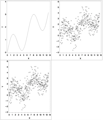
Figure 75.4: Plots for the Curve Fitting Example

PROC TRANSREG increases the squared multiple correlation from the original value of 0.19945 to 0.47062. The plot of T by X shows the original function, the plot of Y by X shows the error-perturbed data, and the third plot shows the data, the true function as a solid curve, and the regression function as the dashed curve. The regression function closely approximates the true function.