Examples
Example 50.1. Segmented Model
From theoretical considerations, you can hypothesize that
That is, for values of x less than x , the equation relating y and x is quadratic (a parabola); and, for values of x greater than x , the equation is constant (a horizontal line). PROC NLIN can fit such a segmented model even when the joint point, x ,is unknown.
The curve must be continuous (the two sections must meet at x ), and the curve must be smooth (the first derivatives with respect to x are the same at x ).
These conditions imply that
The segmented equation includes only three parameters; however, the equation is nonlinear with respect to these parameters.
You can write program statements with PROC NLIN to conditionally execute different sections of code for the two parts of the model, depending on whether x is less than x .
A PUT statement is used to print the constrained parameters every time the program is executed for the first observation (where x = 1). The following statements perform the analysis.
*---------FITTING A SEGMENTED MODEL USING NLIN-----* Y QUADRATIC PLATEAU Y=A+B*X+C*X*X Y=P ..................... . : . : . : . : . : +-----------------------------------------X X0 CONTINUITY RESTRICTION: P=A+B*X0+C*X0**2 SMOOTHNESS RESTRICTION: 0=B+2*C*X0 SO X0=-B/(2*C) *--------------------------------------------------*; title 'Quadratic Model with Plateau'; data a; input y x @@; datalines; .46 1 .47 2 .57 3 .61 4 .62 5 .68 6 .69 7 .78 8 .70 9 .74 10 .77 11 .78 12 .74 13 .80 13 .80 15 .78 16 ; proc nlin; parms a=.45 b=.05 c=-.0025; x0=-.5*b / c; * Estimate join point; if x<x0 then * Quadratic part of Model; model y=a+b*x+c*x*x; else * Plateau part of Model; model y=a+b*x0+c*x0*x0; if _obs_=1 and _iter_ =. then do; plateau=a+b*x0+c*x0*x0; put / x0= plateau= ; end; output out=b predicted=yp; run; /* Setup for creating the graph */ legend1 frame cframe=ligr label=none cborder=black position=center value=(justify=center); axis1 label=(angle=90 rotate=0) minor=none; axis2 minor=none; proc gplot; plot y*x yp*x/frame cframe=ligr legend=legend1 vaxis=axis1 haxis=axis2 overlay ; run;
| |
The NLIN Procedure Dependent Variable y Method: Gauss-Newton x0=12.747669162 plateau=0.7774974276 Sum of Mean Approx Source DF Squares Square F Value Pr > F Model 2 0.1769 0.0884 114.22 <.0001 Error 13 0.0101 0.000774 Corrected Total 15 0.1869 Approx Approximate 95% Confidence Parameter Estimate Std Error Limits a 0.3921 0.0267 0.3345 0.4497 b 0.0605 0.00842 0.0423 0.0787 c 0.00237 0.000551 0.00356 0.00118 Approximate Correlation Matrix a b c a 1.0000000 0.9020250 0.8124327 b 0.9020250 1.0000000 0.9787952 c 0.8124327 0.9787952 1.0000000 x0=12.747669162 plateau=0.7774974276
| |
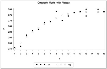
Output 50.1.1 indicates that the join point is 12.75 and the plateau value is 0.78. As displayed in the following plot of the predicted values ( YP ) and the actual values, the selected join point and plateau value is reasonable. The predicted values for the estimation are written to the data set b with the OUTPUT statement.
| |
Quadratic Model with Plateau The NLIN Procedure Dependent Variable y Method: Gauss-Newton Iterative Phase Sum of Iter a b c Squares 0 0.4500 0.0500 0.00250 0.0562 1 0.3881 0.0616 0.00234 0.0118 2 0.3930 0.0601 0.00234 0.0101 3 0.3922 0.0604 0.00237 0.0101 4 0.3921 0.0605 0.00237 0.0101 5 0.3921 0.0605 0.00237 0.0101 6 0.3921 0.0605 0.00237 0.0101 x0=12.747669162 plateau=0.7774974276 NOTE: Convergence criterion met. x0=12.747669162 plateau=0.7774974276
| |
| |
| |
Example 50.2. Iteratively Reweighted Least Squares
The NLIN procedure is suited to methods that make the weight a function of the parameters in each iteration since the _WEIGHT_ variable can be computed with program statements.
The NOHALVE option is used because the SSE definition is modified at each iteration and the step-shortening criteria is thus circumvented.
Iteratively reweighted least squares (IRLS) can produce estimates for many of the robust regression criteria suggested in the literature. These methods act like automatic outlier rejectors since large residual values lead to very small weights. Holland and Welsch (1977) outline several of these robust methods. For example, the biweight criterion suggested by Beaton and Tukey (1974) tries to minimize
where
or
where r is residual / ƒ , ƒ is a measure of scale of the error, and B is a tuning constant.
The weighting function for the biweight is
or
The biweight estimator depends on both a measure of scale (like the standard deviation) and a tuning constant; results vary if these values are changed.
The data are the population of the United States (in millions), recorded at ten-year intervals starting in 1790 and ending in 1990.
title 'U.S. Population Growth'; data uspop; input pop :6.3 @@; retain year 1780; year=year+10; yearsq=year*year; datalines; 3929 5308 7239 9638 12866 17069 23191 31443 39818 50155 62947 75994 91972 105710 122775 131669 151325 179323 203211 226542 248710 ; title 'Beaton/Tukey Biweight Robust Regression using IRLS'; proc nlin data=uspop nohalve; parms b0=20450.43 b1= 22.7806 b2=.0063456; model pop=b0+b1*year+b2*year*year; resid=pop-model.pop; sigma=2; b=4.685; r=abs(resid / sigma); if r<=b then _weight_=(1 (r / b)**2)**2; else _weight_=0; output out=c r=rbi; run; data c; set c; sigma=2; b=4.685; r=abs(rbi / sigma); if r<=b then _weight_=(1 (r / b)**2)**2; else _weight_=0; proc print; run;
| |
Beaton/Tukey Biweight Robust Regression using IRLS The NLIN Procedure Sum of Mean Approx Source DF Squares Square F Value Pr > F Model 2 113564 56782.0 49454.5 <.0001 Error 18 20.6670 1.1482 Corrected Total 20 113585 Approx Approximate 95% Confidence Parameter Estimate Std Error Limits b0 20828.7 259.4 20283.8 21373.6 b1 23.2004 0.2746 23.7773 22.6235 b2 0.00646 0.000073 0.00631 0.00661
| |
Output 50.2.2 displays the computed weights. The observations for 1940 and 1950 are highly discounted because of their large residuals.
| |
Beaton/Tukey Biweight Robust Regression using IRLS Obs pop year yearsq rbi sigma b r _weight_ 1 3.929 1790 3204100 0.93711 2 4.685 0.46855 0.98010 2 5.308 1800 3240000 0.46091 2 4.685 0.23045 0.99517 3 7.239 1810 3276100 1.11853 2 4.685 0.55926 0.97170 4 9.638 1820 3312400 0.95176 2 4.685 0.47588 0.97947 5 12.866 1830 3348900 0.32159 2 4.685 0.16080 0.99765 6 17.069 1840 3385600 0.62597 2 4.685 0.31298 0.99109 7 23.191 1850 3422500 0.94692 2 4.685 0.47346 0.97968 8 31.443 1860 3459600 0.43027 2 4.685 0.21514 0.99579 9 39.818 1870 3496900 1.08302 2 4.685 0.54151 0.97346 10 50.155 1880 3534400 1.06615 2 4.685 0.53308 0.97427 11 62.947 1890 3572100 0.11332 2 4.685 0.05666 0.99971 12 75.994 1900 3610000 0.25539 2 4.685 0.12770 0.99851 13 91.972 1910 3648100 2.03607 2 4.685 1.01804 0.90779 14 105.710 1920 3686400 0.28436 2 4.685 0.14218 0.99816 15 122.775 1930 3724900 0.56725 2 4.685 0.28363 0.99268 16 131.669 1940 3763600 8.61325 2 4.685 4.30662 0.02403 17 151.325 1950 3802500 8.32415 2 4.685 4.16207 0.04443 18 179.323 1960 3841600 0.98543 2 4.685 0.49272 0.97800 19 203.211 1970 3880900 0.95088 2 4.685 0.47544 0.97951 20 226.542 1980 3920400 1.03780 2 4.685 0.51890 0.97562 21 248.710 1990 3960100 1.33067 2 4.685 0.66533 0.96007
| |
Example 50.3. Probit Model with Likelihood function
The data, taken from Lee (1974), consist of patient characteristics and a variable indicating whether cancer remission occurred. This example demonstrates how to use PROC NLIN with a likelihood function. In this case, the likelihood function to minimize is
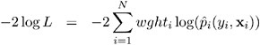
where
and is the normal probability function. This is the likelihood function for a binary probit model. This likelihood is strictly positive so that you can take a square root of ( ![]() i ( y i , x i )) and use this as your residual in PROC NLIN. The DATA step also creates a zero-valued dummy variable, like , that is used as the dependent variable.
i ( y i , x i )) and use this as your residual in PROC NLIN. The DATA step also creates a zero-valued dummy variable, like , that is used as the dependent variable.
Data remiss; input remiss cell smear infil li blast temp; label remiss = 'complete remission'; like = 0; label like = 'dummy variable for nlin'; datalines; 1 .8 .83 .66 1.9 1.1 .996 1 .9 .36 .32 1.4 .74 .992 0 .8 .88 .7 .8 .176 .982 0 1 .87 .87 .7 1.053 .986 1 .9 .75 .68 1.3 .519 .98 0 1 .65 .65 .6 .519 .982 1 .95 .97 .92 1 1.23 .992 0 .95 .87 .83 1.9 1.354 1.02 0 1 .45 .45 .8 .322 .999 0 .95 .36 .34 .5 0 1.038 0 .85 .39 .33 .7 .279 .988 0 .7 .76 .53 1.2 .146 .982 0 .8 .46 .37 .4 .38 1.006 0 .2 .39 .08 .8 .114 .99 0 1 .9 .9 1.1 1.037 .99 1 1 .84 .84 1.9 2.064 1.02 0 .65 .42 .27 .5 .114 1.014 0 1 .75 .75 1 1.322 1.004 0 .5 .44 .22 .6 .114 .99 1 1 .63 .63 1.1 1.072 .986 0 1 .33 .33 .4 .176 1.01 0 0 .9 .93 .84 .6 1.591 1.02 1 1 .58 .58 1 .531 1.002 0 .95 .32 .3 1.6 .886 .988 1 1 .6 .6 1.7 .964 .99 1 1 .69 .69 .9 .398 .986 0 1 .73 .73 .7 .398 .986 ; run; proc nlin data=remiss method=newton sigsq=1; parms a 2 b 1 c 6 int 10; /* Linear portion of model ------*/ eq1 = a*cell + b*li + c*temp +int; /* probit */ p = probnorm(eq1); if (remiss = 1) then p = 1 p; model.like = sqrt( 2 * log(p)); output out=p p=predict; run;
Note that the asymptotic standard errors of the parameters are computed under the least squares assumptions. The SIGSQ=1 option on the PROC NLIN statement forces PROC NLIN to replace the usual mean square error with 1. Also, METHOD=NEWTON is selected so the true Hessian of the likelihood function is used to calculate parameter standard errors rather than the crossproducts approximation to the Hessian.
| |
Beaton/Tukey Biweight Robust Regression using IRLS The NLIN Procedure NOTE: An intercept was not specified for this model. Sum of Mean Approx Source DF Squares Square F Value Pr > F Model 4 21.9002 5.4750 5.75 . Error 23 21.9002 0.9522 Uncorrected Total 27 0 Approx Approximate 95% Confidence Parameter Estimate Std Error Limits a 5.6298 4.6376 15.2234 3.9638 b 2.2513 0.9790 4.2764 0.2262 c 45.1815 34.9095 27.0337 117.4 int 36.7548 32.3607 103.7 30.1879
| |
The problem can be more simply solved using the following SAS statements.
proc probit data=remiss ; class remiss; model remiss=cell li temp ; run;