Some Measurement Models
Psychometric test theory involves many kinds of models relating scores on psychological and educational tests to latent variables representing intelligence or various underlying abilities . The following example uses data on four vocabulary tests from Lord (1957). Tests W and X have 15 items each and are administered with very liberal time limits. Tests Y and Z have 75 items and are administered under time pressure. The covariance matrix is read by the following DATA step:
data lord(type=cov); input _type_ $ _name_ $ w x y z; datalines; n . 649 . . . cov w 86.3979 . . . cov x 57.7751 86.2632 . . cov y 56.8651 59.3177 97.2850 . cov z 58.8986 59.6683 73.8201 97.8192 ;
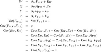
The psychometric model of interest states that W and X are determined by a single common factor F WX , and Y and Z are determined by a single common factor F YZ . The two common factors are expected to have a positive correlation, and it is desired to estimate this correlation. It is convenient to assume that the common factors have unit variance, so their correlation will be equal to their covariance. The error terms for all the manifest variables are assumed to be uncorrelated with each other and with the common factors. The model (labeled here as Model Form D) is as follows .
Model Form D
The corresponding path diagram is as follows.
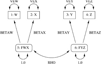
Figure 13.11: Path Diagram: Lord
This path diagram can be converted to a RAM model as follows:
/* 1=w 2=x 3=y 4=z 5=fwx 6=fyz */ title 'H4: unconstrained'; proc calis data=lord cov; ram 1 1 5 betaw, 1 2 5 betax, 1 3 6 betay, 1 4 6 betaz, 2 1 1 vew, 2 2 2 vex, 2 3 3 vey, 2 4 4 vez, 2 5 5 1, 2 6 6 1, 2 5 6 rho; run;
Here are the major results.
| |
H4: unconstrained The CALIS Procedure Covariance Structure Analysis: Maximum Likelihood Estimation Fit Function 0.0011 Goodness of Fit Index (GFI) 0.9995 GFI Adjusted for Degrees of Freedom (AGFI) 0.9946 Root Mean Square Residual (RMR) 0.2720 Parsimonious GFI (Mulaik, 1989) 0.1666 Chi-Square 0.7030 Chi-Square DF 1 Pr > Chi-Square 0.4018 Independence Model Chi-Square 1466.6 Independence Model Chi-Square DF 6 RMSEA Estimate 0.0000 RMSEA 90% Lower Confidence Limit . RMSEA 90% Upper Confidence Limit 0.0974 ECVI Estimate 0.0291 ECVI 90% Lower Confidence Limit . ECVI 90% Upper Confidence Limit 0.0391 Probability of Close Fit 0.6854 Bentler's Comparative Fit Index 1.0000 Normal Theory Reweighted LS Chi-Square 0.7026 Akaike's Information Criterion -1.2970 Bozdogan's (1987) CAIC -6.7725 Schwarz's Bayesian Criterion -5.7725 McDonald's (1989) Centrality 1.0002 Bentler & Bonett's (1980) Non-normed Index 1.0012 Bentler & Bonett's (1980) NFI 0.9995 James, Mulaik, & Brett (1982) Parsimonious NFI 0.1666 Z-Test of Wilson & Hilferty (1931) 0.2363 Bollen (1986) Normed Index Rho1 0.9971 Bollen (1988) Non-normed Index Delta2 1.0002 Hoelter's (1983) Critical N 3543
| |
Figure 13.12: Lord Data: Major Results for RAM Model, Hypothesis H4
| |
H4: unconstrained Covariance Structure Analysis: Maximum Likelihood Estimation RAM Estimates Standard Term Matrix --Row-- -Column- Parameter Estimate Error t Value 1 2 w 1 F1 5 betaw 7.50066 0.32339 23.19 1 2 x 2 F1 5 betax 7.70266 0.32063 24.02 1 2 y 3 F2 6 betay 8.50947 0.32694 26.03 1 2 z 4 F2 6 betaz 8.67505 0.32560 26.64 1 3 E1 1 E1 1 vew 30.13796 2.47037 12.20 1 3 E2 2 E2 2 vex 26.93217 2.43065 11.08 1 3 E3 3 E3 3 vey 24.87396 2.35986 10.54 1 3 E4 4 E4 4 vez 22.56264 2.35028 9.60 1 3 D1 5 D1 5 . 1.00000 1 3 D2 6 D1 5 rho 0.89855 0.01865 48.18 1 3 D2 6 D2 6 . 1.00000
| |
The same analysis can be performed with the LINEQS statement. Subsequent analyses are illustrated with the LINEQS statement rather than the RAM statement because it is slightly easier to understand the constraints as written in the LINEQS statement without constantly referring to the path diagram. The LINEQS and RAM statements may yield slightly different results due to the inexactness of the numerical optimization; the discrepancies can be reduced by specifying a more stringent convergence criterion such as GCONV=1E-4 or GCONV=1E-6. It is convenient to create an OUTRAM= data set for use in fitting other models with additional constraints.
title 'H4: unconstrained'; proc calis data=lord cov outram=ram4; lineqs w=betaw fwx + ew, x=betax fwx + ex, y=betay fyz + ey, z=betaz fyz + ez; std fwx fyz=1, ew ex ey ez=vew vex vey vez; cov fwx fyz=rho; run;
The LINEQS displayed output is as follows.
| |
H4: unconstrained The CALIS Procedure Covariance Structure Analysis: Maximum Likelihood Estimation w = 7.5007*fwx + 1.0000 ew Std Err 0.3234 betaw t Value 23.1939 x = 7.7027*fwx + 1.0000 ex Std Err 0.3206 betax t Value 24.0235 y = 8.5095*fyz + 1.0000 ey Std Err 0.3269 betay t Value 26.0273 z = 8.6751*fyz + 1.0000 ez Std Err 0.3256 betaz t Value 26.6430 Variances of Exogenous Variables Standard Variable Parameter Estimate Error t Value fwx 1.00000 fyz 1.00000 ew vew 30.13796 2.47037 12.20 ex vex 26.93217 2.43065 11.08 ey vey 24.87396 2.35986 10.54 ez vez 22.56264 2.35028 9.60 Covariances Among Exogenous Variables Standard Var1 Var2 Parameter Estimate Error tValue fwx fyz rho 0.89855 0.01865 48.18
| |
Figure 13.13: Lord Data: Using LINEQS Statement for RAM Model, Hypothesis H4
In an analysis of these data by J reskog and S rbom (1979, pp. 54-56; Loehlin 1987, pp. 84-87), four hypotheses are considered :
| H 1 : | = 1, ² W = ² X , Var( E W ) = Var( E X ), ² Y = ² Z , Var( E Y ) = Var( E Z ) |
| H 2 : | same as H 1 : except is unconstrained |
| H 3 : | = 1 |
| H 4 : | Model Form D without any additional constraints |
The hypothesis H 3 says that there is really just one common factor instead of two; in the terminology of test theory, W , X , Y , and Z are said to be congeneric. The hypothesis H 2 says that W and X have the same true-scores and have equal error variance; such tests are said to be parallel. The hypothesis H 2 also requires Y and Z to be parallel. The hypothesis H 1 says that W and X are parallel tests, Y and Z are parallel tests, and all four tests are congeneric.
It is most convenient to fit the models in the opposite order from that in which they are numbered. The previous analysis fit the model for H 4 and created an OUTRAM= data set called ram4 . The hypothesis H 3 can be fitted directly or by modifying the ram4 data set. Since H 3 differs from H 4 only in that is constrained to equal 1, the ram4 data set can be modified by finding the observation for which _NAME_ ='rho' and changing the variable _NAME_ to a blank value (meaning that the observation represents a constant rather than a parameter to be fitted) and setting the variable _ESTIM_ to the value 1. Both of the following analyses produce the same results:
title 'H3: W, X, Y, and Z are congeneric'; proc calis data=lord cov; lineqs w=betawf+ew, x=betaxf+ex, y=betayf+ey, z=betazf+ez; std f=1, ew ex ey ez=vew vex vey vez; run; data ram3(type=ram); set ram4; if _name_='rho' then do; _name_=' '; _estim_=1; end; run; proc calis data=lord inram=ram3 cov; run;
The resulting output from either of these analyses is displayed in Figure 13.14.
| |
H3: W, X, Y, and Z are congeneric The CALIS Procedure Covariance Structure Analysis: Maximum Likelihood Estimation Fit Function 0.0559 Goodness of Fit Index (GFI) 0.9714 GFI Adjusted for Degrees of Freedom (AGFI) 0.8570 Root Mean Square Residual (RMR) 2.4636 Parsimonious GFI (Mulaik, 1989) 0.3238 Chi-Square 36.2095 Chi-Square DF 2 Pr > Chi-Square <.0001 Independence Model Chi-Square 1466.6 Independence Model Chi-Square DF 6 RMSEA Estimate 0.1625 RMSEA 90% Lower Confidence Limit 0.1187 RMSEA 90% Upper Confidence Limit 0.2108 ECVI Estimate 0.0808 ECVI 90% Lower Confidence Limit 0.0561 ECVI 90% Upper Confidence Limit 0.1170 Probability of Close Fit 0.0000 Bentler's Comparative Fit Index 0.9766 Normal Theory Reweighted LS Chi-Square 38.1432 Akaike's Information Criterion 32.2095 Bozdogan's (1987) CAIC 21.2586 Schwarz's Bayesian Criterion 23.2586 McDonald's (1989) Centrality 0.9740 Bentler & Bonett's (1980) Non-normed Index 0.9297 Bentler & Bonett's (1980) NFI 0.9753 James, Mulaik, & Brett (1982) Parsimonious NFI 0.3251 Z-Test of Wilson & Hilferty (1931) 5.2108 Bollen (1986) Normed Index Rho1 0.9259 Bollen (1988) Non-normed Index Delta2 0.9766 Hoelter's (1983) Critical N 109 H3: W, X, Y, and Z are congeneric Covariance Structure Analysis: Maximum Likelihood Estimation w = 7.1047*fwx + 1.0000 ew Std Err 0.3218 betaw t Value 22.0802 x = 7.2691*fwx + 1.0000 ex Std Err 0.3183 betax t Value 22.8397 y = 8.3735*fyz + 1.0000 ey Std Err 0.3254 betay t Value 25.7316 z = 8.5106*fyz + 1.0000 ez Std Err 0.3241 betaz t Value 26.2598 Variances of Exogenous Variables Standard Variable Parameter Estimate Error t Value fwx 1.00000 fyz 1.00000 ew vew 35.92087 2.41466 14.88 ex vex 33.42397 2.31038 14.47 ey vey 27.16980 2.24619 12.10 ez vez 25.38948 2.20839 11.50
| |
Figure 13.14: Lord Data: Major Results for Hypothesis H3
The hypothesis H 2 requires that several pairs of parameters be constrained to have equal estimates. With PROC CALIS, you can impose this constraint by giving the same name to parameters that are constrained to be equal. This can be done directly in the LINEQS and STD statements or by using PROC FSEDIT or a DATA step to change the values in the ram4 data set:
title 'H2: W and X parallel, Y and Z parallel'; proc calis data=lord cov; lineqs w=betawx fwx + ew, x=betawx fwx + ex, y=betayz fyz + ey, z=betayz fyz + ez; std fwx fyz=1, ew ex ey ez=vewx vewx veyz veyz; cov fwx fyz=rho; run;
data ram2(type=ram); set ram4; if _name_='betaw' then _name_='betawx'; if _name_='betax' then _name_='betawx'; if _name_='betay' then _name_='betayz'; if _name_='betaz' then _name_='betayz'; if _name_='vew' then _name_='vewx'; if _name_='vex' then _name_='vewx'; if _name_='vey' then _name_='veyz'; if _name_='vez' then _name_='veyz'; run; proc calis data=lord inram=ram2 cov; run;
The resulting output from either of these analyses is displayed in Figure 13.15.
| |
H2: W and X parallel, Y and Z parallel The CALIS Procedure Covariance Structure Analysis: Maximum Likelihood Estimation Fit Function 0.0030 Goodness of Fit Index (GFI) 0.9985 GFI Adjusted for Degrees of Freedom (AGFI) 0.9970 Root Mean Square Residual (RMR) 0.6983 Parsimonious GFI (Mulaik, 1989) 0.8321 Chi-Square 1.9335 Chi-Square DF 5 Pr > Chi-Square 0.8583 Independence Model Chi-Square 1466.6 Independence Model Chi-Square DF 6 RMSEA Estimate 0.0000 RMSEA 90% Lower Confidence Limit . RMSEA 90% Upper Confidence Limit 0.0293 ECVI Estimate 0.0185 ECVI 90% Lower Confidence Limit . ECVI 90% Upper Confidence Limit 0.0276 Probability of Close Fit 0.9936 Bentler's Comparative Fit Index 1.0000 Normal Theory Reweighted LS Chi-Square 1.9568 Akaike's Information Criterion -8.0665 Bozdogan's (1987) CAIC -35.4436 Schwarz's Bayesian Criterion -30.4436 McDonald's (1989) Centrality 1.0024 Bentler & Bonett's (1980) Non-normed Index 1.0025 Bentler & Bonett's (1980) NFI 0.9987 James, Mulaik, & Brett (1982) Parsimonious NFI 0.8322 Z-Test of Wilson & Hilferty (1931) -1.0768 Bollen (1986) Normed Index Rho1 0.9984 Bollen (1988) Non-normed Index Delta2 1.0021 Hoelter's (1983) Critical N 3712 H2: W and X parallel, Y and Z parallel Covariance Structure Analysis: Maximum Likelihood Estimation w = 7.6010*fwx + 1.0000 ew Std Err 0.2684 betawx t Value 28.3158 x = 7.6010*fwx + 1.0000 ex Std Err 0.2684 betawx t Value 28.3158 y = 8.5919*fyz + 1.0000 ey Std Err 0.2797 betayz t Value 30.7215 z = 8.5919*fyz + 1.0000 ez Std Err 0.2797 betayz t Value 30.7215 Variances of Exogenous Variables Standard Variable Parameter Estimate Error t Value fwx 1.00000 fyz 1.00000 ew vewx 28.55545 1.58641 18.00 ex vewx 28.55545 1.58641 18.00 ey veyz 23.73200 1.31844 18.00 ez veyz 23.73200 1.31844 18.00 Covariances Among Exogenous Variables Standard Var1 Var2 Parameter Estimate Error t Value fwx fyz rho 0.89864 0.01865 48.18
| |
Figure 13.15: Lord Data: Major Results for Hypothesis H2
The hypothesis H 1 requires one more constraint in addition to those in H 2 :
title 'H1: W and X parallel, Y and Z parallel, all congeneric'; proc calis data=lord cov; lineqs w=betawx f + ew, x=betawxf+ex, y=betayzf+ey, z=betayzf+ez; std f=1, ew ex ey ez=vewx vewx veyz veyz; run;
data ram1(type=ram); set ram2; if _name_='rho' then do; _name_=' '; _estim_=1; end; run; proc calis data=lord inram=ram1 cov; run;
The resulting output from either of these analyses is displayed in Figure 13.16.
| |
H1: W and X parallel, Y and Z parallel, all congeneric The CALIS Procedure Covariance Structure Analysis: Maximum Likelihood Estimation Fit Function 0.0576 Goodness of Fit Index (GFI) 0.9705 GFI Adjusted for Degrees of Freedom (AGFI) 0.9509 Root Mean Square Residual (RMR) 2.5430 Parsimonious GFI (Mulaik, 1989) 0.9705 Chi-Square 37.3337 Chi-Square DF 6 Pr > Chi-Square <.0001 Independence Model Chi-Square 1466.6 Independence Model Chi-Square DF 6 RMSEA Estimate 0.0898 RMSEA 90% Lower Confidence Limit 0.0635 RMSEA 90% Upper Confidence Limit 0.1184 ECVI Estimate 0.0701 ECVI 90% Lower Confidence Limit 0.0458 ECVI 90% Upper Confidence Limit 0.1059 Probability of Close Fit 0.0076 Bentler's Comparative Fit Index 0.9785 Normal Theory Reweighted LS Chi-Square 39.3380 Akaike's Information Criterion 25.3337 Bozdogan's (1987) CAIC -7.5189 Schwarz's Bayesian Criterion -1.5189 McDonald's (1989) Centrality 0.9761 Bentler & Bonett's (1980) Non-normed Index 0.9785 Bentler & Bonett's (1980) NFI 0.9745 James, Mulaik, & Brett (1982) Parsimonious NFI 0.9745 Z-Test of Wilson & Hilferty (1931) 4.5535 Bollen (1986) Normed Index Rho1 0.9745 Bollen (1988) Non-normed Index Delta2 0.9785 Hoelter's (1983) Critical N 220 H1: W and X parallel, Y and Z parallel, all congeneric Covariance Structure Analysis: Maximum Likelihood Estimation w = 7.1862*fwx + 1.0000 ew Std Err 0.2660 betawx t Value 27.0180 x = 7.1862*fwx + 1.0000 ex Std Err 0.2660 betawx t Value 27.0180 y = 8.4420*fyz + 1.0000 ey Std Err 0.2800 betayz t Value 30.1494 z = 8.4420*fyz + 1.0000 ez Std Err 0.2800 betayz t Value 30.1494 Variances of Exogenous Variables Standard Variable Parameter Estimate Error t Value fwx 1.00000 fyz 1.00000 ew vewx 34.68865 1.64634 21.07 ex vewx 34.68865 1.64634 21.07 ey veyz 26.28513 1.39955 18.78 ez veyz 26.28513 1.39955 18.78 Covariances Among Exogenous Variables Standard Var1 Var2 Parameter Estimate Error t Value fwx fyz 1.00000
| |
Figure 13.16: Lord Data: Major Results for Hypothesis H1
The goodness-of-fit tests for the four hypotheses are summarized in the following table.
| Hypothesis | Number of Parameters | 2 | Degrees of Freedom | p -value | |
|---|---|---|---|---|---|
| H 1 | 4 | 37.33 | 6 | 0.0000 | 1.0 |
| H 2 | 5 | 1.93 | 5 | 0.8583 | 0.8986 |
| H 3 | 8 | 36.21 | 2 | 0.0000 | 1.0 |
| H 4 | 9 | 0.70 | 1 | 0.4018 | 0.8986 |
The hypotheses H 1 and H 3 , which posit = 1, can be rejected. Hypotheses H 2 and H 4 seem to be consistent with the available data. Since H 2 is obtained by adding four constraints to H 4 , you can test H 2 versus H 4 by computing the differences of the chi-square statistics and their degrees of freedom, yielding a chi-square of 1.23 with four degrees of freedom, which is obviously not significant. So hypothesis H 2 is consistent with the available data.
The estimates of for H 2 and H 4 are almost identical, about 0.90, indicating that the speeded and unspeeded tests are measuring almost the same latent variable, even though the hypotheses that stated they measured exactly the same latent variable are rejected.
EAN: 2147483647
Pages: 156