Relational Operators

We'll begin our examination of relational algebra with the four types of relational operators: restriction, projection, join, and divide. The first two affect a single recordset, although that recordset can, of course, be a view based on any number of other recordsets. The join operator is perhaps the most fundamental to the relational model and defines how two recordsets are to be combined. The final operator, divide, is a rarely used but occasionally handy method of determining which records in one recordset match all the records in a second recordset.

All of these operators are implemented with some form of the SQL SELECT statement. They can be combined in any way you want, subject to the system constraints regarding maximum length and complexity for the statement.

Restriction

The restriction operator returns only those records that meet the specified selection criteria. It is implemented using the WHERE clause of the SELECT statement, as follows:

 SELECT * FROM Employees WHERE LastName = "Davolio"; 

In the Northwind database, this statement returns Nancy Davolio's employee record, since she's the only person in the table with that last name. (The * in the <fieldList> section of the statement is special shorthand for "all fields.")

The selection criteria specified in the WHERE clause can be of arbitrary complexity. Logical expressions can be combined with AND and OR. The expression will be evaluated for each record in the recordset, and if it returns True, that record will be included in the result. If the expression returns either False or Null for the record, it will not be included.

Projection

While restriction takes a horizontal slice of a recordset, projection takes a vertical slice; it returns only a subset of the fields in the original recordset.

SQL performs this simple operation using the <fieldList> section of the SELECT statement by only including the fields that you list. For example, you could use the following statement to create an employee phone list:

 SELECT LastName, FirstName, Extension FROM Employees ORDER BY LastName, FirstName; 

Remember that the ORDER BY clause does just that, it sorts the data; in this case, the list will be sorted alphabetically by the LastName field and then by the FirstName field.

Join

Join operations are probably the most common relational operations. Certainly they are fundamental to the model—it would not be feasible to decompose data into multiple relations were it not possible to recombine it as necessary. This is precisely what a join operator does; it combines recordsets based on the comparison of one or more common fields.

Joins are implemented using the JOIN clause of the SELECT statement. They are categorized based on the type of comparison between the fields involved and the way the results of the comparison are treated. We'll look at each of these in turn.

Equi-Joins

When the join comparison is made on the basis of equality, the join is an equi-join. In an equi-join operation, only those records that have matching values in the specified fields will be returned.

Take, for example, the relations in Figure 5-4. This is a typical case of linked tables resulting from the normalization process. OrderID is the primary key of the Orders table and a foreign key in the Order Details table.

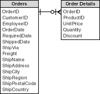
Figure 5-4. These tables can be recombined using the JOIN Operator.

To recombine (and consequently denormalize) the tables, you would use the following SELECT statement:

 SELECT Orders.OrderID, Orders.CustomerID, [Order Details].ProductID FROM Orders INNER JOIN [Order Details] ON Orders.OrderID = [Order Details].OrderID WHERE (((Orders.OrderID)=10248)); 

This statement would result in the recordset shown in Figure 5-5.

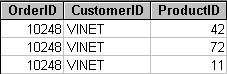
Figure 5-5. This recordset is the result of joining the Orders and Order Details tables.

NOTE

---

If you run this query in Access 2000 using the Northwind database, the result set will show the customer name rather than the CustomerID. This is because Access allows fields to display something other than what's actually stored in them when you declare a lookup control in the table definition. This is a real advantage when Access is used interactively, but wreaks havoc on authors trying to provide examples.

Natural joins

A special case of the equi-join is the natural join. To qualify as a natural join, a join operation must meet the following conditions:

• The comparison operator must be equality.
• All common fields must participate in the join.
• Only one set of common fields must be included in the resulting recordset.

There's nothing intrinsically magical about natural joins. They don't behave in a special manner, nor does the database engine provide special support for them. They are merely the most common form of join, so common that they've been given their own name.

The Jet database engine does do something particularly magical if you create a natural join that meets certain special conditions. If a one-to-many relationship has been established between the two tables, and the common fields included in the view are from the many side of the relationship, then the Jet database engine will perform something called Row Fix-Up or AutoLookup. When the cursor enters the fields used in the join criteria, the Jet database engine will automatically provide the common fields, a spectacular bit of sleight of hand that makes the programmer's life much simpler.

Theta-Joins

Technically, all joins are theta-joins, but by custom, if the comparison operator is equality, the join is always referred to as an equi-join or just as a join. A join based on any other comparison operator (<>, >, >=, <, <=) is a theta-join.

Theta-joins are extremely rare in practice, but they can be handy in solving certain kinds of problems. These problems mostly involve finding records that have a value greater than an average or total, or records that fall within a certain range.

Let's say, for example, that you've created two views, one containing the average number of units sold for each product category and a second containing the total units sold by product, as shown in Figure 5-6. We'll look at how to create these views later in this chapter. For now, just assume their existence.

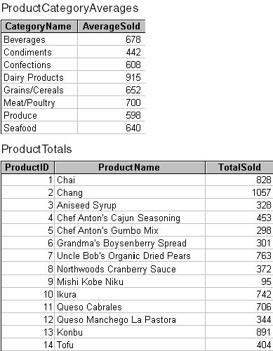
Figure 5-6. These views can be joined using a theta-join.

The following SELECT statement, based on the comparison operator >, will produce a list of the best-selling products within each category:

 SELECT DISTINCTROW ProductCategoryAverages.CategoryName, ProductTotals.ProductName FROM ProductCategoryAverages INNER JOIN ProductTotals ON ProductCategoryAverages.CategoryID = ProductTotals.CategoryID AND ProductTotals.TotalSold > [ProductCategoryAverages].[AverageSold]; 

The results are shown in Figure 5-7.

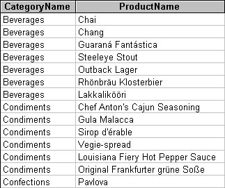
Figure 5-7. This recordset is the result of a theta-join.

In this example, the view could also have been defined using a WHERE clause restriction. In fact, Access will rewrite the query when you leave SQL view to look like the following:

 SELECT DISTINCTROW ProductCategoryAverages.CategoryName, ProductTotals.ProductName FROM ProductCategoryAverages INNER JOIN ProductTotals ON ProductCategoryAverages.CategoryID = ProductTotals.CategoryID WHERE (((ProductTotals.TotalSold)>[ProductCategoryAverages].[AverageSold])); 

Technically, all joins, including equi-joins and natural joins, can be expressed using a restriction. (In database parlance, a theta-join is not an atomic operator.) In the case of theta-joins, this formulation is almost always to be preferred since the database engines are better able to optimize its execution.

Outer joins

All of the joins we've examined so far have been inner joins, joins that return only those records where the join condition evaluates as True. Note that this isn't exactly the same as returning only the records where the specified fields match, although this is how an inner join is usually described. "Match" implies equality, and as we know not all joins are based on equality.

Relational algebra also supports another kind of join, the outer join. An outer join returns all the records returned by an inner join, plus all the records from either or both of the other recordsets. The missing ("unmatched") values will be Null.

Outer joins are categorized as being left, right, or full, depending on which additional records are to be included. Now, when I was in grad school, a left outer join returned all the records from the recordset on the one side of a one-to-many relationship, while a right outer join returned all the records from the many side. For both the Jet database engine and SQL Server, however, the distinction is based on the order in which the recordsets are listed in the SELECT statement. Thus the following two statements both return all the records from X and only those records from Y where the <condition> evaluates to True:

 SELECT * FROM X LEFT OUTER JOIN Y ON <condition> SELECT * FROM Y RIGHT OUTER JOIN X ON <condition> 

A full outer join returns all records from both recordsets, combining those where the condition evaluates as True. SQL Server supports full outer joins with the FULL OUTER JOIN condition:

 SELECT * FROM X FULL OUTER JOIN Y ON <condition> 

The Jet database engine does not directly support full outer joins, but performing a union of a left outer join and a right outer join can duplicate them. We'll discuss unions in the next section.

Divide

The final relational operation is division. The relational divide operator (so called to distinguish it from mathematical division) returns the records in one recordset that have values that match all the corresponding values in the second recordset. For example, given a recordset that shows the categories of products purchased from each supplier, a relational division will produce a list of the suppliers that provide products in all categories.

This is not an uncommon situation, but the solution is not straightforward since the SQL SELECT statement does not directly support relational division. There are numerous ways to achieve the same results as a relational division, however. The easiest method is to rephrase the request.

Instead of "list the suppliers who provide all product categories," which is difficult to process, try "list all suppliers where the count of their product categories is equal to the count of all product categories." This is an example of the extension operation that we'll discuss later in this chapter. It won't always work, and in situations where it doesn't, you can implement division using correlated queries. Correlated queries are, however, outside the scope of this book. Please refer to one of the references listed in the bibliography.