Section 7.3. Aggregate UWB Interference Modeling
|
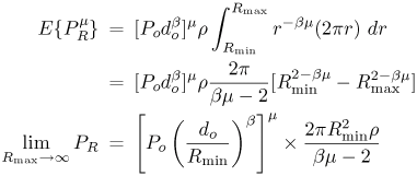
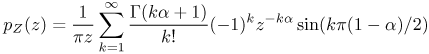
7.3. Aggregate UWB Interference ModelingIn the preceding, we derived detailed expressions for the BER of an NB receiver when subjected to interference from a single UWB emitter. In this section, we consider the aggregate effect due to multiple interferers. We derive a pdf for the asymptotic aggregate interference, which would be useful in a link budget analysis. 7.3.1. Received PowerAlthough narrowband propagation models do not readily apply to the UWB signal (see, for example, [49-51], the propagation channel is well-modeled as linear, and the narrowband propagation model can be applied because the NB receiver only sees a narrowband interfering signal. A gross characterization of the geometric path loss is given by Equation 7.14 where PR denotes the received power at distance d from the source, b is the path loss exponent (typically between 2 and 6), and Po is the power measured at distance do from the transmitter. Consider a single UWB signal, with the Gaussian monocyle pulse, p(t). As we saw earlier, the peak of the UWB signal spectrum is at f =fo. Assuming P (f) is approximately flat over the NB signal bandwidth, [fcWfc +W], with mean power P2(fc) given by (7.3), the interference power due to the UWB pulse is easily found to be Equation 7.15 where PR is the total received power from the UWB source, and h = 2W/fc« 1 for the typical NB receiver. Figure 7.9 shows the normalized interference Figure 7.9. Normalized Interference Versus Normalized Frequency for a Single UWB Interferer into a Victim NB System. The Interference Is Worst When the UWB Spectral Peak Matches the NB Victim Center Frequency.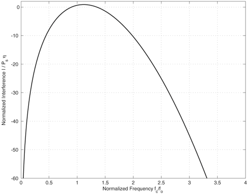 In order to assess the aggregate effect of a number of radios, we consider the following scenario. But it should be noted that the following analysis is not confined to UWB signals. We assume that the receiver uses an omni-directional antenna. The transmitters all have the same transmit power and are uniformly distributed, with density r per square unit, over a concentric ring centered at the receiver with inner and outer radii Rmin and Rmax. Figure 7.10 illustrates this. The uniform distribution implies that the number of transmitters in an area A is Poisson distributed with rate parameter l =rA. The inner ring represents a zone of exclusion and models the minimum separation that one might expect between the radios. The transmitted signals are assumed to be independent of each other. Additionally, it is assumed (although not strictly needed) that all transmitters use the same modulation format. The assumption of equal transmit powers is reasonable in a scheme where power control is difficult. The receiver's basic operation would be to project the received signals onto the signal space, which describes the signal of interest. For example, in a conventional M-ary narrow-band system, this projection would consist of a band-pass filter (BPF), followed by down-conversion to baseband, low-pass filtering to get rid of the double frequency terms, and matched filtering with a bank of filters corresponding to the M waveforms. Figure 7.10. Physical Layout for UWB Aggregate Interference Modeling. The Victim Receiver Is at the Center of the Circle, with Interferers Uniformly Distributed in the Annulus with Inner Radius Rmin and Outer Radius Rmax.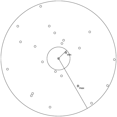 Mean Received PowerThe UWB emitters are randomly located and asynchronous. As such, their complex baseband signals (after front-end processing in the NB receiver) will not be in phase. Because these signals are independent, their powers will add at the receiver. The number of transmitters and their locations, are random; hence, the total received power is also a random variable. With Po denoting received power at reference distance do, as described previously, the expected total power received by the NB radio at the origin from all the transmitters within the annulus is given by Equation 7.16 where we recall that b > 2. In the last equation, the first term describes the received power due to a transmitter at a distance Rmin and the second term describes the aggregate effect due to all the transmitters. Note that because r has dimensions of 1/area, the second term is dimensionless. The term pR2minr represents the effective number of sources within a circle of radius Rmin; the denominator is related to the path loss exponent. Thus, the aggregate effect is represented by a single transmitter at the minimum distance, Rmin, whose received power at the reference point is P'0, given by Equation 7.17 We next consider the moment generating function (MGF). MGF for Received PowerWe just evaluated the expected value of the total received power, PR. One way to characterize the random variable (r.v.) PR is to evaluate its moments. Following the steps leading to (7.16), we obtain for m real, Equation 7.18 where we have assumed that bm > 2. When m = 1, we recover the result in (7.16). Note that the limiting moments do not exist if bm < 2, that is, the lower-order moments, m < 2/b do not exist. This implies that the pdf is very peaked at the origin. The variance of the received power is given by[6]
Equation 7.19 For b Unfortunately this does not lead to a closed-form expression for the pdf.[7]
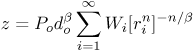
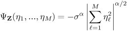
7.3.2. Asymptotic Pdf of Aggregate NoiseWe can conjecture that the aggregate received signal is heavy-tailed. The rationale is that the aggregate of impulsive processes must be impulsive. We establish this analytically. In the preceding, we assumed that the transmitters are Poisson distributed over the plane. Let l denote the Poisson rate parameter and n denote the dimension parameter. Thus n = 2 for sources in the plane, n = 3 for sources in a volume. If l denotes the rate of a n-D homogeneous point process (PP), with points located at distances ri from the origin, Theorem 1 [53, Theorem 1.4.5]. Let {Wi}, and {Gi} be independent sequences of random variables, where Gi is the sequence of arrival times of a unit rate Poisson process. If the Wi are positive valued with E{|W|a} < Equation 7.21 converges almost surely to a positive-valued alpha-stable r.u., with index a, and dispersion parameter sa =E|W|aG(2a)cos(pa/2)/(1a) where G(.) is the Gamma function. The second characteristic function of the r.v. Z is ([53, p. 7]) Equation 7.22 With ri denoting the distances of the Poisson distributed interferers, the total normalized received power is Equation 7.23 The positive-valued random variables Wi represent the effects of shadowing and/or fading, assumed to be independent from transmitter to transmitter. The r.v.s rni are Poisson distributed over [0,
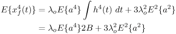
Although a closed-form expression (CFE) for the characteristic function of Z is given in (7.22), a CFE for the pdf exists only when a = 1/2, yielding the Levy distribution whose pdf is [53, p. 10] and cdf is where Q(z) is the tail probability of the standard Gaussian random variable. Recall that if u is a zero-mean unit variance Gaussian r.v., then z can be generated as s/u2. Although the pdf does not exist in closed form for other values of a, a series expansion may be found in [54, Sec XVII.6], Equation 7.24 for 0 < a < 1 and z > 0. From the series expansion, we note that the tails of the pdf decay algebraically as 1/z1+a; as a consequence, E{Zm} < The preceding analysis is an asymptotic one because we assumed that Rmin = 0 (that is, there is no exclusion zone) and that Rmax = It is of interest to compare the pdf of the aggregate interference with that of a single interferer. To this end, we derive the pdf of the location of the nearest interferer. We follow the approach in [41]. The probability that there is no interferer within distance d of the receiver is also the probability that the nearest interferer is distance d away. Because the sources are Poisson distributed with rate r, we have The received power from a source at distance d is PR = Po(do/d)b, where we recall that Po and do are reference values. Thus Pr(PR < z) is the probability that there are no interferers within distance d = do[z/Po]1/b, yielding where we used a = 2/b. For z large, the pdf behaves as 1/z1+a and agrees with the alpha-stable pdf derived for the aggregate interference. In other words, if the scenario is interference limited, the pdf of the interference is adequately described by the nearest interferer that, under the equal transmitted power assumption, dominates the received power. 7.3.3. Amplitudes: Aggregate PdfWe now derive the pdf for the complex amplitude due to the interferers. The received signal passes through the NB receiver's filters; it is converted to complex baseband, and correlated with a bank of M matched filters. Let Ik denote the vector output of the MF bank due to the k-th interferer. Random vector Ik is well-modeled as circularly symmetric zero-mean complex Gaussian. The sources are assumed to be Poisson distributed. The development in [52] is applicable here. The decision variable is now a vector, Equation 7.25 with I being spherically symmetric and alpha-stable, again with index a = 2/b. Note that z is a M-dimensional complex vector due to the M-ary receiver. The joint second characteristic function of this Z is given by Equation 7.26 7.3.4. Bernoulli and Poisson ModelsIn a TH-UWB system, a pulse occupies one of Th chip slots in each frame. The probability of slot occupancy in a given frame is p = 1/Th. If we relax the requirement of one pulse per frame (see the discussion of episodic signaling in Section 7.5) and consider time in units of chip-slot widths, the sequence of pulses constitutes a Bernoulli random process, with probability of occurrence p = 1/Th. In [25], we had considered this model briefly. If p is small, the normalized kurtosis, Equation 7.27 indicating that the interference is strongly non-Gaussian. This non-Gaussianity can be exploited to estimate the frequency-selective channel encountered by the UWB signal. The k-th order normalized cumulants are roughly p1 k/2. A limiting case is the Poisson process model. Let tk denote the arrival times of the UWB pulses at a receiver. Given that the UWB signals are time-hopped, episodic, and asynchronous, it is reasonable to model the pulse times as the arrival times of a Poisson process. The effects of multipaths can be included in this model. To facilitate analysis, let us assume that the delays and amplitudes associated with each path are independent of one another, and identically distributed. Let l(t) denote the rate (pulses per second) of this inhomogeneous Poisson process (IPP), tk the arrival times, ak the amplitudes, and p Such a model is called a marked point process (MPP) with multiplicative marks. The marks are the random variables, the aks. This is a special case of an MPP that we had considered in [58]. More recently, an unmarked homogeneous point process (HPP) model (ak In an NB receiver, the signal x(t) would be filtered. If the bandwidth of the NB system is small relative to that of x(t), it is reasonable to model the FT's of the individual pulses pk(t) to be flat over the NB system's band-pass region, [fc W, fc + W]. Thus, the effective signal can be represented as Equation 7.29 where hnb(t) denotes the NB receive filter. The cumulants of this process are given by [58, eq. (9)] [59] Equation 7.30 For a HPP, l(t) If h(t) is band-pass, H(0) = 0, and E{xf (t)} = 0. The variance is given by Equation 7.32 for a receive filter with unit energy. The kurtosis is given by Equation 7.33 This in turn yields the power at the output of an envelope detector Equation 7.34 which follows readily from 7.3.5. Simulation Examples
|
 0. Hence, we will not pursue this approach.
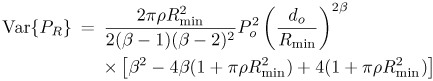
 2 (corresponding to some reported indoor applications with LOS), some of the lower-order integer moments may not exist. For
  , for some (0, 1), we can conclude as a special case of [53, Theorem 1.4.5] that the random variable
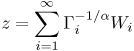

 1) was considered in [60].
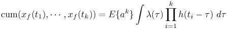

 2 is the path loss exponent. Let
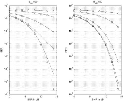
|
EAN: 2147483647
Pages: 110