Using Analysis Services Data Mining Tools to Solve Problems in Business Scenarios

The following section discusses various scenarios and technical situations in which you may find yourself. The goal of these scenarios is to go beyond basic step-by-steps of how to use the designers or wizards, and to provide tips and insights about some non-obvious capabilities of our designers and wizards. The scenarios that you are presented within this section are listed here by tool:

• Data Mining Designer

  • Embedding Data Mining controls and sample code in a custom application

  • Interpreting the "Little Diamonds" and how to view them

  • Recoding a column, using the Data Source View

  • Measuring lift over global statistics

  • Creating a Classification Matrix Report

  • Enhancing productivity by multi-selecting in the Data Mining Wizard and Editor in BI Development Studio

  • Using Association rules viewer filtering capability

  • Using the same base column multiple times with different properties in different algorithms (discretized for some, continuous for others)

  • Creating multiple models, using the same algorithm but varying column setting (Input, Predict) or changing properties

  • Copying grid and trees viewers in Microsoft Excel, Microsoft Word, or HTML

  • Using the DMX editor to call the stored procedure to display the data contained in the viewers

• SQL Server Management Studio:

  • Viewing and customizing DMX templates

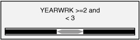
How to Embed Data Mining Controls and Sample Code in a Custom Application

In Analysis Services 2000, the data mining offering consisted of two algorithms and three viewers. These viewers couldn't be reused outside of Analysis Manager.

In Analysis Services 2005, the Data Mining offering has been greatly enhanced. The Analysis Services engine now natively supports ten algorithms, and it also contains ten different viewers. The other main difference is that each of these viewers was natively built as components that can be reused and embedded in other applications.

This is particularly important because many of the usage scenarios for data mining are part of an existing application. The value-add of data mining techniques is to make decisions easier for the user by providing extra insight into the data. Thus, data mining is rarely a standalone application, but rather functionality that is embedded in another application.

The following sample illustrates how to embed such functionality in a C# application:

 // Determine the viewer type based on the model service and // instantiate the correct viewer model = conn.MiningModels[modelName]; service = conn.MiningServices[model.Algorithm]; if (service.ViewerType == "Microsoft_Cluster_Viewer")       viewer = new ClusterViewer(); else if (service.ViewerType == "Microsoft_Tree_Viewer")       viewer = new TreeViewer(); else if (service.ViewerType == "Microsoft_NaiveBayesian_Viewer")       viewer = new NaiveBayesViewer(); else if (service.ViewerType ==                "Microsoft_SequenceCluster_Viewer")       viewer = new SequenceClusterViewer(); else if (service.ViewerType == "Microsoft_TimeSeries_Viewer")       viewer = new TimeSeriesViewer(); else if (service.ViewerType ==                "Microsoft_AssociationRules_Viewer")       viewer = new AssociationViewer(); else if (service.ViewerType == "Microsoft_NeuralNetwork_Viewer")       viewer = new NeuralNetViewer(); else throw new System.Exception("Custom Viewers not supported"); // Set up and load the viewer viewer.ConnectionString = ConnectionString; viewer.MiningModelName = modelName; viewer.Dock = DockStyle.Fill; panel.Controls.Add(viewer); viewer.LoadViewerData(null); 

The full sample, as well as many others, can be found on the following data mining website, managed by the Microsoft SQL Server Data Mining development team:

http://www.sqlserverdatamining.com/DMCommunity/Downloads/default.aspx

How to Interpret "Little Diamonds" and How to View Them

The Cluster, Regression Tree, and Time Series viewers use small cyancolored diamond shapes in their nodes and rowsets.

Figure 14-1 show one such node, for example.

Figure 14-1. Cluster node illustrating use of little diamond.

We use graphics of this sort for quick visual representation of continuous distributions.

The first thing to note is that the size of the "diamond" symbol is proportional to the standard deviation of the target variable, so the bigger the node diamond, the greater the uncertainty of the predictions based on that node.

Another thing to notice is that in some contexts the diamond is off-center, that is, displaced from the middle of the supporting black bar in either direction, such as in the Cluster viewer snippet shown in Figure 14-2.

Figure 14-2. Example of cluster viewer snippet.

The supporting black bar represents the range of a continuous variable distribution, and its middle corresponds to the population median (same as marginal mean for normal distribution). The center of a diamond represents a category-specific or node-specific mean and the displacement is proportional to the difference between the two means. Thus in Figure 14.2, the average income of the population in Cluster 8 is above the median, but for Cluster 2 it is below the median. Judging from the displacements, neither of the clusters diverges very far from the population-wide statistical average. However, Cluster 2 shows much greater variation in income than Cluster 8. The range of the black bar is equal to the range of the input data but capped at three standard deviations away from the mean. This is to prevent outliers from skewing the data view and making it meaningless.

The numerical details of the distribution involved are readily accessible from the Mining Legend. The diamond symbols are designed to give just a first-glance impression of the data mining statistics.

Recoding a Column Using the Data Source View

Many times when embarking on a data mining project you need to slightly alter the data source. We're not talking about changing the world; rather we want to look at the data in a subtly but significantly different manner so that it makes more sense to the business problem under examination. In these cases you may need to reduce or change the number of states in a column to those that make sense for your business problem, or change a numeric value into a set of discrete states.

Nominal Recoding

For example, imagine that for your modeling purposes you determine that you need to know the legal marital status of each customer. However, your data has a column called Marital Status with the following values:

• Never Married

• Married

• Separated

• Divorced

• Widowed

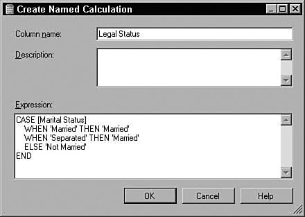
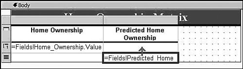
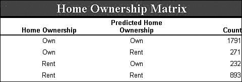
Clearly this column does not suit your purposes. What you need is a different column that simply has the values Married and Not Married. Luckily, using the Data Source View editor, you can add such a column without modifying your source data or even touching your source database.

The Data Source View (DSV) enables you to add logical columns to the physical columns in your source tables. To the Analysis Services processing engine, these columns appear the same as any physical column in the table. To create such a column, right-click on a table in the DSV editor and select New Named Calculation, which brings up the Create (per Figure) Named Calculation dialog. In this dialog you can enter arbitrary SQL that generates the appropriate values for your column. For recoding, we use the SQL CASE statement to change values from one set to another. The CASE statement looks like the following:

CASE <expression>    WHEN <value> THEN <value>    [WHEN <value> THEN <value>]    [ELSE <value>] END 

For the Marital Status example, the statement would look like this:

CASE [Marital Status]     WHEN 'Married' THEN 'Married'     WHEN 'Separated' THEN 'Married'     ELSE 'Not Married' END 

To create the Named Calculation, you fill out the Create Named Calculation dialog with the new column name and the SQL fragment, as shown in Figure 14-3.

Figure 14-3. Creating a named calculation.

You may also want only to change the column values in some of the cases. For example, if you want to recode the married values into a single value, but preserve all the non-married states, you could use a CASE statement like the following:

CASE [Marital Status]     WHEN 'Married' THEN 'Married'     WHEN 'Separated' THEN 'Married'     ELSE [Marital Status] END 

Numerical Recoding

The other type of recoding mentioned involves recoding a numerical value into a set of discrete states. For this purpose you use a different form of the CASE statement:

CASE   WHEN <expression> THEN <value>   [WHEN <expression> THEN <value>]   [ELSE <value>] END 

For example, if you wanted to know whether people were in their twenties or thirties you could use the following SQL expression:

CASE   WHEN [Age] >= 20 AND [Age] < 30 THEN 'Twenties'   WHEN [Age] >= 30 AND [Age] < 50 THEN 'Thirties'   ELSE 'Other' END 

Verifying Recoding

Verifying your recoding is simple. To see the data that Analysis Services uses to process your model, right-click on the table in the DSV editor and select Explore Data. The data viewers use the same mechanism used by the server to pull data from the source, so your data exploration includes the named calculations you added.

Measuring Lift over Global Statistics

One of the typical methods to validate a model is to measure the accuracy of the trained model in terms of correct classification rate. To facilitate this, Analysis Services 2005 supports a lift chart where prediction accuracy of a model is compared with an ideal model and random model. Figure 14-4 presents an example.

Figure 14-4. Data Mining lift chart.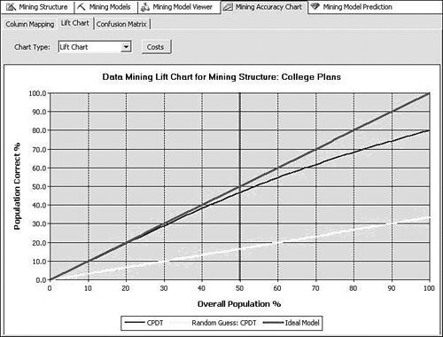

The chart shows that the model called CPDT significantly outperforms random prediction, which is 0.33 because the target has three states (missing, Yes, No). However, this chart doesn't tell how much better the CPDT model is than marginal prediction (that is, prediction based on just global distribution of the target). What if the global distribution of the target being "Yes" is 85%? As far as the correct classification rate is concerned, the marginal prediction would be better (note that CPDT yields 80% overall). This is why sometimes we also need to know how much the model performs better than marginal. To include a marginal model in the lift chart, you can create a derived model with only the target and key included and all other columns ignored. Figure 14-5 shows the derived model, named CPMG.

Figure 14-5. Example of a derived model.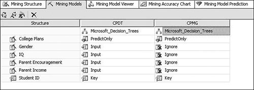

Now, try the lift chart with the two models, named CPDT and CPMG, to show lift over the marginal model (see Figure 14-6).

Figure 14-6. Lift chart with two mining models.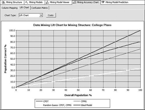

Creating a Classification Matrix Report

Reporting Services makes an excellent delivery vehicle for your data mining results. In addition to exposing query results, you can also use features of Reporting Services to enhance the functionality of DMX. For example, DMX lacks GROUP BY functionality, so you can take advantage of the Reporting Services grouping capability in data mining reports.

Using this capability you can easily emulate the classification matrix functionality of the BI Development Studio in a report that you can deliver to anyone. The first thing you need is a mining model that predicts a discrete attribute and test data. For this example I use a decision tree model built on the movie customer data available on this site to show a classification matrix (also known as a confusion matrix) for the Home Ownership column.

The first thing to do is to create a new Reporting Services project and connect to your Analysis Services database containing your model. When you generate your query, you select the actual column from the test data set and the predicted column from the model. It's a good idea to give the predicted column a name. For example, if your test data column is Home Ownership, then you might call your predicted column Predicted Home Ownership, as shown in Figure 14-7.

Figure 14-7. Data mining query in Reporting Services.

When you set up the grouping levels for your report, put the actual value (e.g., Home Ownership) into the group box and the predicted value (e.g., Predicted Home Ownership) into the details box. In the end, we want both items in the group, but Reporting Services requires that you put something in the details in the wizard, so you can move Predicted Home Ownership to the group box later.

After you finish the Report Wizard, edit the report layout to move Predicted Home Ownership from the details line to the grouping line, as shown in Figure 14-8. Then you can delete the details row from the report.

Figure 14-8. Moving Predicted Home Ownership from the details line to the grouping line.

Next, right-click the grouping icon to the left of the row and select Edit Group. Add Predicted Home Ownership to the list of grouping fields and click OK.

Finally, you need to add a new column to the report. For the column header you can type Count and for the cell value enter =CountRows(). Your final layout should look something like that shown in Figure 14-9 (with some additional formatting):

Figure 14-9. Report preview.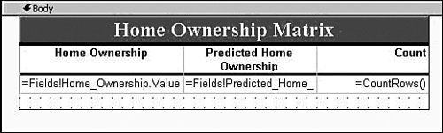

Preview your report and you will receive a thin-client, distributable, portable, classification matrix like the one shown in Figure 14-10.

Figure 14-10. Report Design final layout.

How Multi-Selecting in the Data Mining Wizard and Editor in BI Development Studio Can Enhance Productivity

Several places in SQL Server 2005 Business Intelligence Development Studio support multi-selection of objects, which lets you set the state of many objects at the same time. This can be quite useful in the following scenarios:

• In the Data Mining Wizard, when selecting which columns are input and\or predictable, you can click (use the arrow keys) to position the selection in a cell, then while holding down the Shift key, either scroll and click on another cell to select a range of cells, or use the arrow keys. The cells in the table are all shaded to show that they are all selected. To set the state, press the space bar. Pressing the space bar again toggles the check boxes and un-checks them.

• In the Data Mining Editor's mining structure view, you cannot multi-select columns in the tree to set common properties in the property sheet grid at the same time. However, because the structure columns also appear in the Mining Models view in the leftmost column of the grid, you can multi-select the structure columns there by holding down the Shift key while making the selection and then set properties on several of the structure columns at the same time. Press F4 to show the property sheet if it is not already visible, or choose to show it from the View menu. This can be useful when changing several mining structure columns' content type, for example, from discrete to continuous.

• In addition to setting common properties with the property sheet in the Mining Models view, you can also multi-select cells in the mining models grid to set the usage type for several mining model columns and several models all at once. Use the Shift key again to select multiple cells. To activate the combo-box drop-down while retaining the multiple-selection state, press the F2 key. Select the usage type and commit the value. The value is then set across the entire selection.

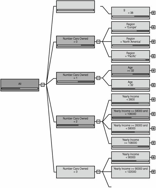
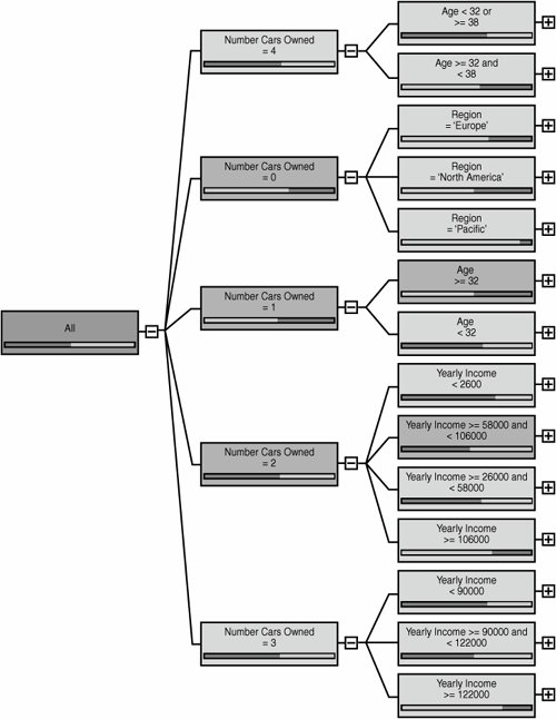
Using Association Rules Viewer Filtering Capability

The association rule algorithm is useful because it can help with detecting association patterns in the data. For example, the very first rule shown in Figure 14-11 can be read as follows: People who buy ML Road Tire and Sport-100 are likely to buy the Road Tire Tube as well with 100% probability.

Figure 14-11. Association rule, unfiltered.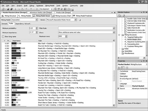

Using the AdventureWorks sample cube project, you can browse an association rule mining model called Market Basket. It shows association patterns in the Bicycle Sales data.

An association Mining Model can contain many rules. Because of the high volume, the filter capability is most relevant. A very basic and common filtering is to type a string in the filter dialog.

For example, if you type: "Road Tire" in the Filter combo box, you reduce the number of rules to just 20, which makes it much easier to read and analyze (see Figure 14-12).

Figure 14-12. Simple association rule filter.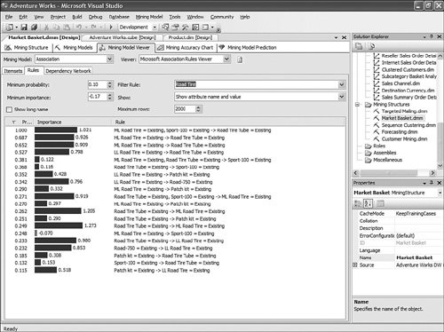

But what is not often known is that the Microsoft Association Rules Viewer filtering is based on a .NET regular expression. As a result, the filtering supports more than just wildcards and and/or logic. It also supports all the types of .NET regular expressions, as described at the following page: http://msdn.microsoft.com/library/default.asp?url=/library/en-us/cpgenref/html/cpconregularexpressionslanguageelements.asp.

For example, the following filtering expression finds rules having the phrase "Road Tire Tube" on the left side of the rule: \bRoad\b.\bTire\b.\bTube\b.*->*, resulting in what is shown in Figure 14-13.

Figure 14-13. Advanced association rule filter.

Use the Same Base Column Multiple Times with Different Properties in Different Algorithms

There are many scenarios in which it can be interesting and useful to use the same input list of columns, but with different properties.

For example, some algorithms allow only discrete states (not continuous), such as Naïve Bayes. In other cases, a column may need to be treated as discretized into five buckets for one mining model algorithm (for example: decision tree model), and eight buckets for another model. Creating multiple mining models within the same mining structure allows you to compare how treating this input with a finer granularity of discretization affects the models.

You can create as many model variations as needed.

In Figure 14-14, Yearly Income has been left continuous, whereas Yearly Income 1 has been added from the same base column, but with the Content properties set to discretized in ten buckets.

Figure 14-14. DM use of multiple similar base columns.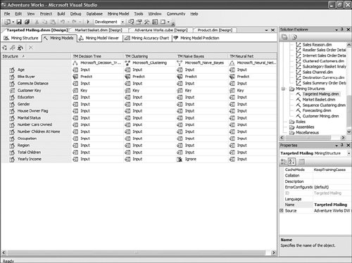

Creating Multiple Models, Using the Same Algorithm but with Varying Column Settings or Changing Properties

Although most people create a mining structure with multiple models (each one using a different technique), there might be scenarios where it is relevant and useful to use the same Mining Model technique with different combinations of input, predict settings, or properties settings for base columns.

For example, using the same algorithm for two models, if you predict college plans using only Age as input, you get different results than you do if you use Parent Income and Parent Encouragement. A third algorithm that uses all the available columns as input produces different results, as well. Sometimes when there are potentially a lot of columns to choose from, you may not need to use 100 or more columns all as input to train the model. You can discover which columns are those that are most correlated with the predictable attribute and then build additional models that narrow down the scope of important columns. In this case you could build the structure with all those columns and then try different combinations by including some inputs and not others.

Copying Grid and Trees Viewers in Microsoft Excel, Microsoft Word, or HTML

Most of the Data Mining viewers are very graphical. Often the graphical shape and overall look of the tree or layout of the cluster distribution can provide as much information as the content itself. This is why each viewer allows you to copy the graphical information to the clipboard and then paste it to Excel, Word, or even a rich format.

The user can use the shortcut key Ctrl+C or right-click on the viewer and use one of the context menu options:

• Copy Graph view, which copies the graph in its current state (see Figure 14-15).

  Figure 14-15. Copy Graph view.

  

• Copy Entire Graph, which copies the graph entirely, expanded and displayed (see Figure 14-16).

  Figure 14-16. Copy entire graph.

  

DMX Editor Can Call the Stored Proc to Display the Data Contained in the Viewers

This is a slightly more advanced topic. The Data Mining tools make use of many internal stored procedures to query mining model content and display it inside the viewers. These stored procedures can also be used and invoked by the database administrator directly through the DMX query editor in SQL Server Management Studio to query the content of a mining model.

In the following example, the following query queries the first 20 node definitions of the TM Decision Tree Mining Model from the AdventureWorks DW Analysis Services sample:

[View full width]
Call System.Microsoft.AnalysisServices.System.DataMining.DecisionTree sDepNet.  DTGetNodeGraph('TM Decision Tree', 20) 

The results of the query can be seen in Figure 14-17.

Figure 14-17. Using Stored Procedure to navigate Data Mining Model content.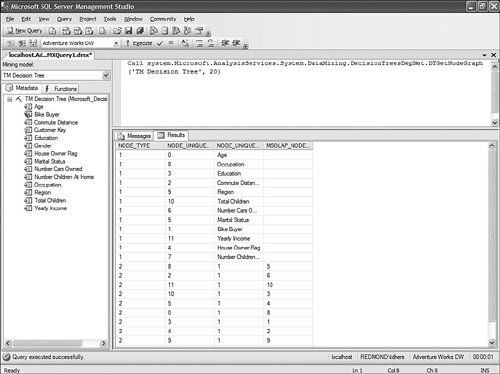

The full list of available stored procedures, as well as their definitions, can be found in Appendix D.

How to View and Customize DMX Templates

In SQL Server Management Studio, go to View, Template Explorer. The default view shows standard SQL templates. Click the "Cube" icon in the window to get to the Analysis Services templates and open the DMX branch of the tree. There you will find many template DMX syntax examples (see Figure 14-18).

Figure 14-18. Analysis Services Template Explorer.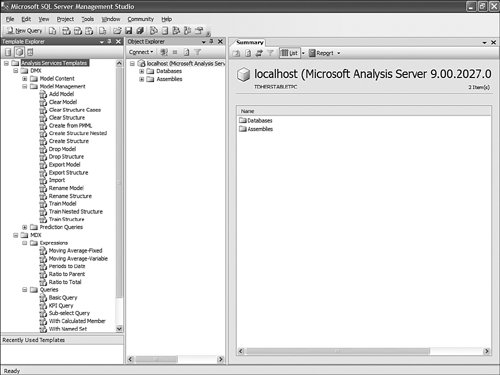

For example, the "Base Prediction" template gives you the following shellfill in the parameters and you have a valid prediction query:

// ========================== // Base Prediction // ========================== SELECT <select_list,,> FROM <mining_model,,> PREDICTION JOIN OPENQUERY('<datasource,,>','<query,,>') AS <input_alias,,> ON <on_clause,,> WHERE <where_clause,,> 

This template list is stored on disc in a clear XML file under C:\Program Files\Microsoft SQL Server\90\Tools\Binn\VSShell\Common7\IDE\sqlworkbenchprojectitems\AnalysisServices.

As with KPI templates and other time intelligence templates, one can easily open any of the XML documents stored in the sub-folders and edit, add, or remove templates. Unlike KPI templates, each query or expression template is stored in a different file; to add a template, create an XML file with the MDX, DXM, or XML/A expression and save it in the appropriate sub-folder.

The MDX, DMX, XML/A folder structure is shown in Figure 14-19.

Figure 14-19. DMX template folder structure.