INCOMPLETE MEASURES

A measure is a value in the base data that the multidimensional database will aggregate at each point in the hierarchy. In this section we outline the problems posed by three of the kinds of incomplete information that could appear in a measure attribute: unknown values, imprecise values, and probabilistic values. The techniques proposed to manage the incomplete information are adaptable to other kinds of incompleteness.

Unknown Measure Values

Unknown values will be the most common kind of incomplete information in a multidimensional database. The reason is that the base data is often stored in an SQL-compliant database, and only one kind of incomplete information is supported in SQL: null values. A null value in SQL usually represents either an unknown value or an inapplicable value (Melton & Simon, 1993). Many real-world datasets have null values. SQL is not very adept at dealing with null values in aggregate operations; it discards null values in aggregates (in effect treating them as inapplicable values).

To illustrate techniques for dealing with unknown values in the base data for a multidimensional database, assume that the protein attribute of a Nutrition tuple for Fuji apples is an unknown value. The incomplete information indicates that Fuji apples have some amount of protein, but it is unknown exactly how much. The problem is how to best utilize the unknown value, while remaining sensitive to the limited knowledge provided by the value.

There are several strategies for computing the maximum protein and counting the overall amount of protein for apples with an unknown amount of protein. The strategies are discussed below and illustrated in Figure 3. In each part of the figure, two base data facts and a single base node are shown. The base node measures the maximum amount of protein among products sold.

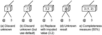
Figure 3: Options for Handling an Unknown Value (in a Max Aggregate)

Discard the unknown value: This strategy is to throw out the incomplete information rather than using it, which is the default SQL behavior for aggregates. The advantage of this technique is that it is extremely simple and efficient. All multidimensional database products can implement the strategy with no loss of efficiency. Figure 3(a) shows the idea. The unknown value is represented by a ‘@’ character.

One disadvantage of discarding unknown values is that the technique will likely produce semantically incorrect information. The unknown value that is discarded could be the maximum or could be a non-zero quantity in a summation. Another problem occurs when all the base data is unknown. Consider the case of computing the maximum protein for Fuji apples shown in Figure 3(b). The base node needs to store the max protein for Fuji apples. Unfortunately, there is no such value since the amount of protein is unknown for all the base data. Some number, however, must be inserted, so a reasonable default value is used. The obvious candidate is a negative number. The negative number is a good choice since complete information about an amount of protein will always be zero or greater. So when points higher in the hierarchy are needed, e.g., get the maximum protein over all fruits, the negative values (incomplete information) will be discarded in favor of non-negative ones (complete information). For sum aggregates, a default value of zero would be used. A user will have to correctly interpret any spurious replacement values that appear in a result, but the technique is simple to implement.

Replace with an imputed value: Imputation is the process of using other information to estimate an unknown value. Techniques for imputing missing values are common in statistics. A standard method is to use a mean or median value. For example, the mean amount of protein in other kinds of apples is 3.2 grams of protein, so 3.2 could be imputed for Fuji apples that have unknown values. Figure 3(c) shows an example of replacing the unknown with the mean.

Imputing a value could be a more complex computation that depends on the values of other attributes and additional metadata about the unknown value. For example, assume that apples have a color attribute, which can be the value red, green, or yellow. Fuji apples are green. Available metadata about green apples states that they lack a color-dependent gene found in red apples that produces protein. Other metadata about apples includes the knowledge that the amount of protein is within 20% of the amount of vitamin C in an apple. So the amount of protein in Fuji apples is computed as an estimate of the lower bound of the amount in red apples, scaled by a factor of the amount of vitamin C. The primary advantage of imputation is that it produces a statistically meaningful replacement value, as opposed to a non-statistical default value. A second advantage is that in an eager implementation, the cost of imputing a value is incurred at most once.

One disadvantage of imputation is that an imputed value is typically an average, mean, median, or expectation rather than an extreme value, so it would have no effect on a max/min aggregate. A second disadvantage is that in spite of the availability of metadata for imputing values in many applications, especially in the health-related industries, no database product that we are aware of offers any support for using metadata to impute values. Such support would further degrade the performance of lazy multidimensional databases since the imputation is done during query evaluation. A third disadvantage is that the imputed value is given the same status within the hierarchy as a non-imputed value (both are just numbers), but in reality we have less confidence in the imputed value. This can be remedied by storing the method of imputation and a value representing the degree of confidence in the result along with the imputed value. But the multidimensional database must then have some technique for handling confidence values in the hierarchy. Finally, the use of imputation will often mean that the variance of the data will be artificially small, since the imputed values most often do not contribute to the variance. This can be solved by using multiple imputation (Rubin, 1987), where imputation is performed in a number of separate passes, the results of which are then combined into the overall result.

Generate an unknown result: An unknown value is used as the result. Computing a max on an unknown value would result in an unknown answer as shown in Figure 3(d). This pushes the problem up the hierarchy.

Measure the completeness: The ratio of unknown-to-known values is used as a measure of the completeness of the result. Different notions of completeness have been advanced, but a common notion is that the completeness is a percentage of the known values used to compute an aggregate. An aggregate computed entirely on known values has 100% completeness, while one computed half of unknown values has a completeness of 50%. An alternative method of computing completeness is to weight the alternatives. Note that the completeness can be added to the multidimensional database as a measure; it is a count of known values and unknown values. Figure 3(e) shows the computation of a completeness measure for a max aggregate. The completeness is represented in parentheses next to the value as a pair of the count of known values and all values. If the multidimensional database treats the completeness as a measure, it can be computed easily for derived nodes. However, the measure should be displayed to the user as a percentage.

Imprecise Measure Values

The handling of imprecise values differs slightly from unknown values. An imprecise value is a sequence of potential values. In the sense that it represents a set of potential values, one of which is the actual value, it is similar to an unknown value. The key difference is that the imprecise value may possibly map to somewhere below top in the hierarchy in each dimension, since the hierarchy is effectively a precision hierarchy. So there is often a point in the hierarchy above at which the imprecise value is completely known. For example, a date of July 1, 2001, is imprecise with respect to a category of hours since it spans 24 potential hours. But the date is complete information at the category of days, since the exact day is known.

One source of imprecise values is a data warehouse that integrates several data sources. Normally, the data warehouse cleanses or scrubs the data prior to insertion. One aspect of cleansing is to remove category mismatches among the data sources by mapping the data to the coarsest category. For example, if the time of sale from one source is given in hours, while that of a second source is given in days, then the hourly data is scrubbed by mapping each hour to the day that contains it. The scrubbing makes "time of sale" data uniform across the data sources, so that the data can be inserted into the data warehouse. The drawback is that some information is discarded during the data scrubbing. An alternative strategy is to record imprecise values. Each day can be represented as an imprecise value of 24 hours.

The following techniques can be used to handle imprecise values. They are similar to those for unknown values, but include extra conditions to manage the mapping of the imprecise value to some precise location in the hierarchy. Figure 4 illustrates the techniques. The figure assumes that a max aggregate is being performed on an imprecisely known amount of protein in two varieties of apple.

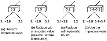
Figure 4: Options for Handling an Imprecise Value (in a Max Aggregate)

Discard the imprecise value: Same as for unknown values. This alternative is not a very good one for imprecise values because an imprecise value is more complete than an unknown value. Figure 4(a) shows the strategy. The imprecise value is discarded, along with the information that the amount of protein might be larger than 3.2.

Replace with an imputed value, default value, or a randomly sampled value: Imputation can be more accurate for imprecise values because the set of potential values is smaller. Imputation metadata for an imprecise value would typically include a probability distribution over the range of potential values. The probability distribution could be used to impute the expected value. In Figure 4(b) the expected value, 3.5, is used to replace the imprecise value. It happens to be the maximum. Expected values are unappealing for extreme value aggregates like max and min. An alternative is to use random sampling. In random sampling, the probability distribution is used to select a potential value. The randomly chosen value is used instead of the expected value. In aggregation, for large numbers of imprecise values, random sampling has the same desirable effect as imputing the expected value, since the values will average out to the expected value. But random sampling will produce extreme values that are absent when imputing the expected value. Since values are chosen randomly, however, the same aggregate computed on the same data twice in succession may yield different results.

Replace with a "bound": An imprecise value is a range of potential values, from a least potential value to a greatest potential value. For max and sum aggregates, a "pessimistic" choice would be to replace the imprecise value with the least potential value. An "optimistic" choice would be to use the greatest potential value. For a min aggregate the choices would be reversed. In Figure 4(c) the greatest potential value is chosen, and it turns out to be the maximum.

The advantage of all the replacement strategies is that the replacement value is a complete value, so the implementation is simple and the rest of the multidimensional database does not change. The disadvantage is that no matter what choice is made, some useful information is lost because the underlying data value is imprecise.

Use the imprecise value: The aggregate uses the imprecise value to compute an imprecise result. The bounds are computed by interval arithmetic. As the category becomes coarser, the imprecision will gradually reduce until it eventually disappears. Figure 4(d) depicts an example of computing the bounds. Two imprecise values are compared, and the maximum of the lower and upper bounds are propagated into the result.

Probabilistic (and Possibilistic) Values in the Data

A probabilistic value in the data is a weighted, exclusive, disjunctive value. The weights provide additional information about which potential values are more likely, but change the management of the incomplete information only slightly from that for unweighted values.

Replace with an imputed value: As discussed in the handling of imprecise values, it is natural to use the probabilities to impute an expected value or to use random sampling to select a potential value. In aggregation, for large numbers of probabilistic values, random sampling has the same desirable effect as imputing the expected value, since the values will average out to the expected value. But random sampling will produce extreme values that are absent when imputing the expected value.

Use a probabilistic value: Bayesian probability theory has sound formulas for computing the count, max, min, and sum of probabilistic values. The drawback is that the formulas have relatively high space and time complexity. For a set of n probabilistic values, each with m potential values, the worst-case time and space cost to compute an aggregate is O(mⁿ).

The handling of possibilistic values, which are weighted inclusive disjunctive values, is similar to that of probabilistic values.