4.2 VOICE

---

4.2 VOICE

To transmit voice from one place to another, the speech (acoustic signal) is first converted into an electrical signal using a transducer, the microphone. This electrical signal is an analog signal. The voice signal corresponding to the speech "how are you" is shown in Figure 4.1. The important characteristics of the voice signal are given here:

• The voice signal occupies a bandwidth of 4kHz i.e., the highest frequency component in the voice signal is 4kHz. Though higher frequency components are present, they are not significant, so a filter is used to remove all the high-frequency components above 4kHz. In telephone networks, the bandwidth is limited to only 3.4kHz.

• The pitch varies from person to person. Pitch is the fundamental frequency in the voice signal. In a male voice, the pitch is in the range of 50–250 Hz. In a female voice, the pitch is in the range of 200–400 Hz.

• The speech sounds can be classified broadly as voiced sounds and unvoiced sounds. Signals corresponding to voiced sounds (such as the vowels a, e, i, o, u) will be periodic signals and will have high amplitude. Signals corresponding to unvoiced sounds (such as th, s, z, etc.) will look like noise signals and will have low amplitude.

• Voice signal is considered a nonstationary signal, i.e., the characteristics of the signal (such as pitch and energy) vary. However, if we take small portions of the voice signals of about 20msec duration, the signal can be considered stationary. In other words, during this small duration, the characteristics of the signal do not change much. Therefore, the pitch value can be calculated using the voice signal of 20msec. However, if we take the next 20msec, the pitch may be different.

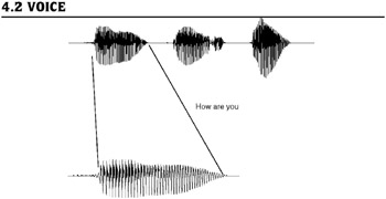
Figure 4.1: Speech waveform.

The voice signal occupies a bandwidth of 4KHz. The voice signal can be broken down into a fundamental frequency and its harmonics. The fundamental frequency or pitch is low for a male voice and high for a female voice.

These characteristics are used while converting the analog voice signal into digital form. Analog-to-digital conversion of voice signals can be done using one of two techniques: waveform coding and vocoding.

Note 

The characteristics of speech signals described here are used extensively for speech processing applications such as text-to-speech conversion and speech recognition.

Music signals have a bandwidth of 20kHz. The techniques used for converting music signals into digital form are the same as for voice signals.

4.2.1 Waveform Coding

Waveform coding is done in such a way that the analog electrical signal can be reproduced at the receiving end with minimum distortion. Hundreds of waveform coding techniques have been proposed by many researchers. We will study two important waveform coding techniques: pulse code modulation (PCM) and adaptive differential pulse code modulation (ADPCM).

Pulse Code Modulation

Pulse Code Modulation (PCM) is the first and the most widely used waveform coding technique. The ITU-T Recommendation G.711 specifies the algorithm for coding speech in PCM format.

PCM coding technique is based on Nyquist's theorem, which states that if a signal is sampled uniformly at least at the rate of twice the highest frequency component, it can be reconstructed without any distortion. The highest frequency component in voice signal is 4kHz, so we need to sample the waveform at 8000 samples per second—every 1/8000th of a second (125 microseconds). We have to find out the amplitude of the waveform for every 125 microseconds and transmit that value instead of transmitting the analog signal as it is. The sample values are still analog values, and we can "quantize" these values into a fixed number of levels. As shown in Figure 4.2, if the number of quantization levels is 256, we can represent each sample by 8 bits. So, 1 second of voice signal can be represented by 8000 × 8 bits, 64kbits. Hence, for transmitting voice using PCM, we require 64 kbps data rate. However, note that since we are approximating the sample values through quantization, there will be a distortion in the reconstructed signal; this distortion is known as quantization noise.

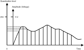
Figure 4.2: Pulse Code Modulation.

ITU-T standard G.711 specifies the mechanism for coding of voice signals. The voice signal is band limited to 4kHz, sampled at 8000 samples per second, and each sample is represented by 8 bits. Hence, using PCM, voice signals can be coded at 64kbps.

In the PCM coding technique standardized by ITU in the G.711 recommendation, the nonlinear characteristic of human hearing is exploited— the ear is more sensitive to the quantization noise in the lower amplitude signal than to noise in the large amplitude signal. In G.711, a logarithmic (non-linear) quantization function is applied to the speech signal, and so the small signals are quantized with higher precision. Two quantization functions, called A-law and m-law, have been defined in G.711. m-law is used in the U.S. and Japan. A-law is used in Europe and the countries that follow European standards. The speech quality produced by the PCM coding technique is called toll quality speech and is taken as the reference to compare the quality of other speech coding techniques.

For CD-quality audio, the sampling rate is 44.1kHz (one sample every 23 microseconds), and each sample is coded with 16 bits. For two-channel stereo audio stream, the bit rate required is 2 × 44.1 × 1000 × 16 = 1.41Mbps.

Note 

The quality of speech obtained using the PCM coding technique is called toll quality. To compare the quality of different coding techniques, toll quality speech is taken as the reference.

Adaptive Differential Pulse Code Modulation

One simple modification that can be mode to PCM is that we can code the difference between two successive samples rather than coding the samples directly. This technique is known as differential pulse code modulation (DPCM).

Another characteristic of the voice signal that can be used is that a sample value can be predicted from past sample values. At the transmitting side, we predict the sample value and find the difference between the predicted value and the actual value and then send the difference value. This technique is known as adaptive differential pulse code modulation (ADPCM). Using ADPCM, voice signals can be coded at 32kbps without any degradation of quality as compared to PCM.

ITU-T Recommendation G.721 specifies the coding algorithm. In ADPCM, the value of speech sample is not transmitted, but the difference between the predicted value and the actual sample value is. Generally, the ADPCM coder takes the PCM coded speech data and converts it to ADPCM data.

The block diagram of an ADPCM encoder is shown in Figure 4.3(a). Eight-bit [.mu]-law PCM samples are input to the encoder and are converted into linear format. Each sample value is predicted using a prediction algorithm, and then the predicted value of the linear sample is subtracted from the actual value to generate the difference signal. Adaptive quantization is performed on this difference value to produce a 4-bit ADPCM sample value, which is transmitted. Instead of representing each sample by 8 bits, in ADPCM only 4 bits are used. At the receiving end, the decoder, shown in Figure 4.3(b), obtains the dequantized version of the digital signal. This value is added to the value generated by the adaptive predictor to produce the linear PCM coded speech, which is adjusted to reconstruct m-law-based PCM coded speech.

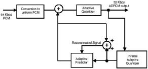
Figure 4.3: (a) ADPCM Encoder.

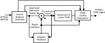
Figure 4.3: (b) ADPCM Decoder.

There are many waveform coding techniques such as delta modulation (DM) and continuously variable slope delta modulation (CVSD). Using these, the coding rate can be reduced to 16kbps, 9.8kbps, and so on. As the coding rate reduces, the quality of the speech is also going down. There are coding techniques using good quality speech which can be produced at low coding rates.

The PCM coding technique is used extensively in telephone networks. ADPCM is used in telephone networks as well as in many radio systems such as digital enhanced cordless telecommunications (DECT).

In ADPCM, each sample is represented by 4 bits, and hence the data rate required is 32kbps. ADPCM is used in telephone networks as well as radio systems such as DECT.

Note 

Over the past 50 years, hundreds of waveform coding techniques have been developed with which data rates can be reduced to as low as 9.8kbps to get good quality speech.

4.2.2 Vocoding

A radically different method of coding speech signals was proposed by H. Dudley in 1939. He named his coder vocoder, a term derived from VOice CODER. In a vocoder, the electrical model for speech production seen in Figure 4.4 is used. This model is called the source–filter model because the speech production mechanism is considered as two distinct entities—a filter to model the vocal tract and an excitation source. The excitation source consists of a pulse generator and a noise generator. The filter is excited by the pulse generator to produce voiced sounds (vowels) and by the noise generator to produce unvoiced sounds (consonants). The vocal tract filter is a time-varying filter—the filter coefficients vary with time. As the characteristics of the voice signal vary slowly with time, for time periods on the order of 20msec, the filter coefficients can be assumed to be constant.

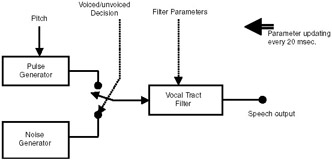
Figure 4.4: Electrical model of speech production.

In vocoding techniques, at the transmitter, the speech signal is divided into frames of 20msec in duration. Each frame contains 160 samples. Each frame is analyzed to check whether it is a voiced frame or unvoiced frame by using parameters such as energy, amplitude levels, etc. For voiced frames, the pitch is determined. For each frame, the filter coefficients are also determined. These parameters—voiced/unvoiced classification, filter coefficients, and pitch for voiced frames—are transmitted to the receiver. At the receiving end, the speech signal is reconstructed using the electrical model of speech production. Using this approach, the data rate can be reduced as low as 1.2kbps. However, compared to voice coding techniques, the quality of speech will not be very good. A number of techniques are used for calculating the filter coefficients. Linear prediction is the most widely used of these techniques.

In vocoding techniques, the electrical model of speech production is used. In this model, the vocal tract is represented as a filter. The filter is excited by a pulse generator to produce voiced sounds and by a noise generator to produce unvoiced sounds.

Note 

The voice generated using the vocoding techniques sounds very mechanical or robotic. Such a voice is called synthesized voice. Many speech synthesizers, which are integrated into robots, cameras, and such, use the vocoding techniques.

Linear Prediction

The basic concept of linear prediction is that the sample of a voice signal can be approximated as a linear combination of the past samples of the signal.

If S_n is the n^th speech sample, then

where a_k (k = 1,…,P) are the linear prediction coefficients, G is the gain of the vocal tract filter, and U_n is the excitation to the filter. Linear prediction coefficients (generally 8 to 12) represent the vocal tract filter coefficients. Calculating the linear prediction coefficients involves solving P linear equations. One of the most widely used methods for solving these equations is through the Durbin and Levinson algorithm.

Coding of the voice signal using linear prediction analysis involves the following steps:

• At the transmitting end, divide the voice signal into frames, each frame of 20msec duration. For each frame, calculate the linear prediction coefficients and pitch and find out whether the frame is voiced or unvoiced. Convert these values into code words and send them to the receiving end.

• At the receiver, using these parameters and the speech production model, reconstruct the voice signal.

In linear prediction technique, a voice sample is approximated as a linear combination of the past n samples. The linear prediction coefficients are calculated every 20 milliseconds and sent to the receiver, which reconstructs the speech samples using these coefficients. Using this approach, voice signals can be compressed to as low as 1.2kbps.

Using linear prediction vocoder, voice signals can be compressed to as low as 1.2kbps. Quality of speech will be very good for data rates down to 9.6kbps, but the voice sounds synthetic for further lower data rates. Slight variations of this technique are used extensively in many practical systems such as mobile communication systems, speech synthesizers, etc.

Note 

Variations of LPC technique are used in many commercial systems, such as mobile communication systems and Internet telephony.

---