6.1 The SELECT Statement
|
| < Day Day Up > |
|
It is always faster to SELECT exact column names. Thus using the Employees schema
SELECT division_id, name, city, state, country FROM division;
is faster than
SELECT * FROM division;
Also since there is a primary key index on the Division table
SELECT division_id FROM division;
will only read the index file and should completely ignore the table itself. Since the index contains only a single column and the table contains five columns, reading the index is faster because there is less physical space to traverse.
In order to prove these points we need to use the EXPLAIN PLAN command. Oracle Database's EXPLAIN PLAN command allows a quick peek into how the Oracle Database Optimizer will execute an SQL statement, displaying a query plan devised by the Optimizer.
The EXPLAIN PLAN command creates entries in the PLAN_TABLE for a SELECT statement. The resulting query plan for the SELECT statement following is shown after it. Various versions of the query used to retrieve rows from the PLAN_TABLE, a hierarchical query, can be found in Appendix B. In order to use the EXPLAIN PLAN command statistics must be generated. Both the EXPLAIN PLAN command and statistics will be covered in detail in Chapter 9.
EXPLAIN PLAN SET statement_id='TEST' FOR SELECT * FROM division; Query Cost Rows Bytes ----------------------------------- ---- ---- ----- SELECT STATEMENT on 1 10 460 TABLE ACCESS FULL on DIVISION 1 10 460
One thing important to remember about the EXPLAIN PLAN command is it produces a listed sequence of events, a query plan. Examine the following query and its query plan. The "Pos" or positional column gives a rough guide to the sequence of events that the Optimizer will follow. In general, events will occur listed in the query plan from bottom to top, where additional indenting denotes containment.
EXPLAIN PLAN SET statement_id='TEST' FOR SELECT di.name, de.name, prj.name, SUM(prj.budget-prj.cost) FROM division di JOIN department de USING(division_id) JOIN project prj USING(department_id) GROUP BY di.name, de.name, prj.name HAVING SUM(prj.budget-prj.cost) > 0; Query Pos Cost Rows Bytes ---------------------------------- --- ---- ---- ----- SELECT STATEMENT on 97 97 250 17500 FILTER on 1 SORT GROUP BY on 1 97 250 17500 HASH JOIN on 1 24 10000 700000 TABLE ACCESS FULL on DIVISION 1 1 10 170 HASH JOIN on 2 3 100 3600 TABLE ACCESS FULL on DEPARTMENT 1 1 100 1900 TABLE ACCESS FULL on PROJECT 2 13 10000 340000
Now let's use the Accounts schema. The Accounts schema has some very large tables. Large tables show differences between the costs of data retrievals more easily. The GeneralLedger table contains over 700,000 rows at this point in time.
In the next example, we explicitly retrieve all columns from the table using column names, similar to using SELECT * FROM GeneralLedger. Using the asterisk probably involves a small overhead in re-interpretation into a list of all column names, but this is internal to Oracle Database and unless there are a huge number of these types of queries this is probably negligible.
EXPLAIN PLAN SET statement_id='TEST' FOR SELECT generalledger_id,coa#,dr,cr,dte FROM generalledger;
The cost of retrieving 752,740 rows is 493 and the GeneralLedger table is read in its entirety indicated by "TABLE ACCESS FULL".
Query Cost Rows Bytes ----------------------------------- ---- ------ -------- SELECT STATEMENT on 493 752740 19571240 TABLE ACCESS FULL on GENERALLEDGER 493 752740 19571240
Now we will retrieve only the primary key column from the GeneralLedger table.
EXPLAIN PLAN SET statement_id='TEST' FOR SELECT generalledger_id FROM generalledger;
For the same number of rows the cost is reduced to 217 since the byte value is reduced by reading the index only, using a form of a full index scan. This means that only the primary key index is being read, not the table.
Query Cost Rows Bytes ------------------------------------------------ ------ -------- SELECT STATEMENT on 217 752740 4516440 INDEX FAST FULL SCAN on XPKGENERALLEDGER 217 752740 4516440
Here is another example using an explicit column name but this one has a greater difference in cost from that of the full table scan. This is because the column retrieved uses an index, which is physically smaller than the index for the primary key. The index on the COA# column is consistently 5 bytes in length for all rows. For the primary key index only the first 9,999 rows have an index value of less than 5 bytes in length.
EXPLAIN PLAN SET statement_id='TEST' FOR SELECT coa# FROM generalledger; Query Cost Rows Bytes ---------------------------------- ---- ------ ------- SELECT STATEMENT on 5 752740 4516440 INDEX FAST FULL SCAN on XFK_GL_COA# 5 752740 4516440
Following are two interesting examples utilizing a composite index. The structure of the index is built as the SEQ# column contained within the CHEQUE_ID column (CHEQUE_ID + SEQ#) and not the other way around. In older versions of Oracle Database this probably would have been a problem. The Oracle9i Database Optimizer is now much improved when matching poorly ordered SQL statement columns to existing indexes. Both examples use the same index. The order of columns is not necessarily a problem in Oracle9i Database.
| Note | Oracle Database 10 Grid Oracle Database 10g has Optimizer improvements such as less of a need for SQL code statements to be case sensitive. |
EXPLAIN PLAN SET statement_id='TEST' FOR SELECT cheque_id, seq# FROM cashbookline; Query Cost Rows Bytes --------------------------------------- ---- ------ ------- SELECT STATEMENT on 65 188185 1505480 INDEX FAST FULL SCAN on XPKCASHBOOKLINE 65 188185 1505480
It can be seen that even with the columns selected in the reverse order of the index, the index is still used.
EXPLAIN PLAN SET statement_id='TEST' FOR SELECT seq#,cheque_id FROM cashbookline; Query Cost Rows Bytes ---------------------------------- ---- ------ ------- SELECT STATEMENT on 65 188185 1505480 INDEX FAST FULL SCAN on XPKCASHBOOKLINE 65 188185 1505480
The GeneralLedger table has a large number of rows. Now let's examine the idiosyncrasies of very small tables. There are some differences between the behavior of SQL when dealing with large and small tables.
In the next example, the Stock table is small and thus the costs of reading the table or the index are the same. The first query, doing the full table scan, reads around 20 times more physical space but the cost is the same. When tables are small the processing speed may not be better when using indexes. Additionally when joining tables the Optimizer may very well choose to full scan a small static table rather than read both index and table. The Optimizer may select the full table scan as being quicker. This is often the case with generic static tables containing multiple types since they are typically read more often.
EXPLAIN PLAN SET statement_id='TEST' FOR SELECT * FROM stock; Query Cost Rows Bytes ---------------------------------- ---- ---- ----- SELECT STATEMENT on 1 118 9322 TABLE ACCESS FULL on STOCK 1 118 9322 EXPLAIN PLAN SET statement_id='TEST' FOR SELECT stock_id FROM stock; Query Cost Rows Bytes ---------------------------------- ---- ---- ----- SELECT STATEMENT on 1 118 472 INDEX FULL SCAN on XPKSTOCK 1 118 472
So that is a brief look into how to tune simple SELECT statements. Try to use explicit columns and try to read columns in index orders if possible, even to the point of reading indexes and not tables.
6.1.1 A Count of Rows in the Accounts Schema
I want to show a row count of all tables in the Accounts schema I have in my database. If you remember we have already stated that larger tables are more likely to require use of indexes and smaller tables are not. Since the Accounts schema has both large and small tables, SELECT statements and various clauses executed against different tables will very much affect how those different tables should be accessed in the interest of good performance. Current row counts for all tables in the Accounts schema are shown in Figure 6.1.
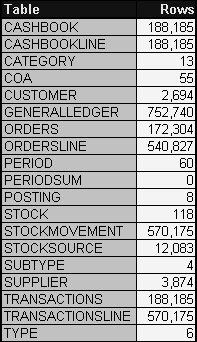
Figure 6.1: Row Counts of Accounts Schema Tables
| Tip | Accounts schema row counts vary throughout this book since the database is continually actively adding rows and occasionally recovered to the initial state shown in Figure 6.1. Relative row counts between tables remain constant. |
6.1.2 Filtering with the WHERE Clause
Filtering the results of a SELECT statement with a WHERE clause implies retrieving only a subset of rows from a larger set of rows. The WHERE clause can be used to either include wanted rows, exclude unwanted rows or both.
Once again using the Employees schema, in the following SQL statement we filter rows to include only those rows we want, retrieving only those rows with PROJECTTYPE values starting with the letter "R".
SELECT * FROM projecttype WHERE name LIKE 'R%';
Now we do the opposite and filter out rows we do not want. We get everything with values not starting with the letter "R".
SELECT * FROM projecttype WHERE name NOT LIKE 'R%';
How does the WHERE clause affect the performance of a SELECT statement? If the sequence of expression comparisons in a WHERE clause can match an index it should. The WHERE clause in the SELECT statement above does not match an index and thus the whole table will be read. Since the Employees schema ProjectType table is small, having only 11 rows, this is unimportant. However, in the case of the Accounts schema, where many of the tables have large numbers of rows, avoiding full table scans, and forcing index reading is important. Following is a single WHERE clause comparison condition example SELECT statement. We will once again show the cost of the query using the EXPLAIN PLAN command. This query does an exact match on a very large table by applying an exact value to find a single row. Note the unique index scan and the low cost of the query.
EXPLAIN PLAN SET statement_id='TEST' FOR SELECT * FROM stockmovement WHERE stockmovement_id = 5000; Query Cost Rows Bytes ---------------------------------- ---- ------ ----- SELECT STATEMENT on 3 1 24 TABLE ACCESS BY INDEX ROWID on STOCKMOVEMENT 3 1 24 INDEX UNIQUE SCAN on XPKSTOCKMOVEMENT 2 1
Now let's compare the query above with an example which uses another single column index but searches for many more rows than a single row. This example consists of two queries. The first query gives us the WHERE clause literal value for the second query. The result of the first query is displayed here.
SQL> SELECT coa#, COUNT(coa#) "Rows" FROM generalledger GROUP BY coa#; COA# Rows ----- -------------- 30001 310086 40003 66284 41000 173511 50001 169717 60001 33142
Now let's look at a query plan for the second query with the WHERE clause filter applied. The second query shown next finds all the rows in one of the groups listed in the result shown above.
EXPLAIN PLAN SET statement_id='TEST' FOR SELECT * FROM generalledger WHERE coa# = 40003; Query Cost Rows Bytes ---------------------------------- ---- ------ ------- SELECT STATEMENT on 493 150548 3914248 TABLE ACCESS FULL on GENERALLEDGER 493 150548 3914248
The query above has an interesting result because the table is fully scanned. This is because the Optimizer considers it more efficient to read the entire table rather than use the index on the COA# column to find specific columns in the table. This is because the WHERE clause will retrieve over 60,000 rows, just shy of 10% of the entire GeneralLedger table. Over 10% is enough to trigger the Optimizer to execute a full table scan.
In comparison to the above query the following two queries read a very small table, the first with a unique index hit, and the second with a full table scan as a result of the range comparison condition (<). In the second query, if the table were much larger possibly the Optimizer would have executed an index range scan and read the index file. However, since the table is small the Optimizer considers reading the entire table as being faster than reading the index to find what could be more than a single row.
EXPLAIN PLAN SET statement_id='TEST' FOR SELECT * FROM category WHERE category_id = 1; Query Cost Rows Bytes ---------------------------------- ---- ---- ----- SELECT STATEMENT on 1 1 12 TABLE ACCESS BY INDEX ROWID on CATEGORY 1 1 12 INDEX UNIQUE SCAN on XPKCATEGORY 1 EXPLAIN PLAN SET statement_id='TEST' FOR SELECT * FROM category WHERE category_id < 2;
The costs of both index use and the full table scan are the same because the table is small.
Query Cost Rows Bytes ---------------------------------- ---- ---- ----- SELECT STATEMENT on 1 1 12 TABLE ACCESS FULL on CATEGORY 1 1 12
So far we have looked at WHERE clauses containing single comparison conditions. In tables where multiple column indexes exist there are other factors to consider. The following two queries produce exactly the same result. Note the unique index scan on the primary key for both queries. As with the ordering of index columns in the SELECT statement, in previous versions of Oracle it is possible that the same result would not have occurred for the second query. This is because in the past the order of table column comparison conditions absolutely had to match the order of columns in an index. In the past the second query shown would probably have resulted in a full table scan. The Optimizer is now more intelligent in Oracle9i Database.
| Note | Oracle Database 10 Grid Oracle Database 10g has Optimizer improvements such as less of a need for SQL code statements to be case sensitive. |
We had a similar result previously in this chapter using the CHEQUE_ID and SEQ# columns on the CashbookLine table. The same applies to the WHERE clause.
EXPLAIN PLAN SET statement_id='TEST' FOR SELECT * FROM ordersline WHERE order_id = 3137 AND seq# = 1; Query Cost Rows Bytes ---------------------------------- ---- ---- ----- SELECT STATEMENT on 3 1 17 TABLE ACCESS BY INDEX ROWID on ORDERSLINE 3 1 17 INDEX UNIQUE SCAN on XPKORDERSLINE 2 1 EXPLAIN PLAN SET statement_id='TEST' FOR SELECT * FROM ordersline WHERE seq# = 1 AND order_id= 3137; Query Cost Rows Bytes ---------------------------------- ---- ---- ----- SELECT STATEMENT on 3 1 17 TABLE ACCESS BY INDEX ROWID on ORDERSLINE 3 1 17 INDEX UNIQUE SCAN on XPKORDERSLINE 2 1
Let's now try a different variation. The next example query should only use the second column in the composite index on the STOCK_ID and SUPPLIER_ID columns on the StockSource table. What must be done first is to find a StockSource row uniquely identified by both the STOCK_ID and SUPPLIER_ID columns. Let's simply create a unique row. I have not used sequences in the INSERT statements shown because I want to preserve the values of the sequence objects.
| Tip | The names of the columns in the Stock table Stock.MIN and Stock.MAX refer to minimum and maximum Stock item values in the Stock table, not the MIN and MAX Oracle SQL functions. |
INSERT INTO stock(stock_id, category_id, text, min, max) VALUES((SELECT MAX(stock_id)+1 FROM stock),1,'text',1,100); INSERT INTO supplier(supplier_id, name, ticker) VALUES((SELECT MAX(supplier_id)+1 FROM supplier) ,'name','TICKER'); INSERT INTO stocksource VALUES((SELECT MAX(supplier_id) FROM supplier) ,(SELECT MAX(stock_id) FROM stock),100.00);
The INSERT statements created a single row in the StockSource table with the primary key composite index uniquely identifying the first column, the second column, and the combination of both. We can find those unique values by finding the maximum values for them.
SELECT COUNT(stock_id), MAX(stock_id) FROM stocksource WHERE stock_id = (SELECT MAX(stock_id) FROM stocksource) GROUP BY stock_id; COUNT(STOCK_ID) MAX(STOCK_ID) --------------- --------------- 1 119 SELECT COUNT(supplier_id), MAX(supplier_id) FROM stocksource WHERE supplier_id = (SELECT MAX(supplier_id) FROM supplier) GROUP BY supplier_id; COUNT(SUPPLIER_ID) MAX(SUPPLIER_ID) ------------------ ---------------- 1 3875
Now let's attempt that unique index hit on the second column of the composite index in the StockSource table, amongst other combinations.
EXPLAIN PLAN SET statement_id='TEST' FOR SELECT * FROM stocksource WHERE supplier_id = 3875;
Something very interesting happens. The foreign key index on the SUPPLIER_ID column is range scanned because the WHERE clause is matched. The composite index is ignored.
Query Cost Rows Bytes --------------------------------------- ---- ---- ----- 1. SELECT STATEMENT on 2 3 30 2. TABLE ACCESS BY INDEX ROWID on STOCKSOURCE 2 3 30 3. INDEX RANGE SCAN on XFK_SS_SUPPLIER 1 3
The following query uses the STOCK_ID column, the first column in the composite index. Once again, even though the STOCK_ID column is the first column in the composite index the Optimizer matches the WHERE clause against the nonunique foreign key index on the STOCK_ID column. Again the result is a range scan.
EXPLAIN PLAN SET statement_id='TEST' FOR SELECT * FROM stocksource WHERE stock_id = 119; Query Cost Rows Bytes ------------------------------------- ---- ---- ----- 1. SELECT STATEMENT on 8 102 1020 2. TABLE ACCESS BY INDEX ROWID on STOCKSOURCE 8 102 1020 3. INDEX RANGE SCAN on XFK_SS_STOCK 1 102
The next query executes a unique index hit on the composite index because the WHERE clause exactly matches the index.
EXPLAIN PLAN SET statement_id='TEST' FOR SELECT * FROM stocksource WHERE stock_id = 119 AND supplier_id = 3875; Query Cost Rows Bytes ----------------------------------------- ---- ----- ----- 1. SELECT STATEMENT on 2 1 10 2. TABLE ACCESS BY INDEX ROWID on STOCKSOURCE 2 1 10 3. INDEX UNIQUE SCAN on XPK_STOCKSOURCE 1 12084
Let's clean up and delete the unique rows we created with the INSERT statements above. My script executing queries (see Appendix B) on the PLAN_TABLE contains a COMMIT command and thus ROLLBACK will not work.
DELETE FROM StockSource WHERE supplier_id = 3875 and stock_id = 119; DELETE FROM supplier WHERE supplier_id = 3875; DELETE FROM stock WHERE stock_id = 119; COMMIT;
Now let's do something slightly different. The purpose of creating unique stock and supplier items in the StockSource table was to get the best possibility of producing a unique index hit. If we were to select from the StockSource table where more than a single row existed we would once again not get unique index hits. Depending on the number of rows found we could get index range scans or even full table scans.
Firstly, find maximum and minimum counts for stocks duplicated on the StockSource table.
SELECT * FROM( SELECT supplier_id, COUNT(supplier_id) AS suppliers FROM stocksource GROUP BY supplier_id ORDER BY suppliers DESC) WHERE ROWNUM = 1 UNION SELECT * FROM( SELECT supplier_id, COUNT(supplier_id) AS suppliers FROM stocksource GROUP BY supplier_id ORDER BY suppliers) WHERE ROWNUM = 1;
There are nine suppliers with a SUPPLIER_ID column value of 2711 and one with SUPPLIER_ID column value 2.
SUPPLIER_ID SUPPLIERS ------------- ------------- 2 1 2711 9
Both the next two queries perform index range scans. If one of the queries retrieved enough rows, as in the COA# = '40003' previously shown in this chapter, the Optimizer would force a read of the entire table.
EXPLAIN PLAN SET statement_id='TEST' FOR SELECT * FROM stocksource WHERE supplier_id = 2; Query Cost Rows Bytes --------------------------------------- ---- ---- ----- 1. SELECT STATEMENT on 2 3 30 2. TABLE ACCESS BY INDEX ROWID on STOCKSOURCE 2 3 30 3. INDEX RANGE SCAN on XFK_SS_SUPPLIER 1 3 EXPLAIN PLAN SET statement_id='TEST' FOR SELECT * FROM stocksource WHERE supplier_id = 2711; Query Cost Rows Bytes --------------------------------------- ---- ---- ----- 1. SELECT STATEMENT on 2 3 30 2. TABLE ACCESS BY INDEX ROWID on STOCKSOURCE 2 3 30 3. INDEX RANGE SCAN on XFK_SS_SUPPLIER 1 3
So try to always do two things with WHERE clauses. Firstly, try to match comparison condition column sequences with existing index column sequences, although it is not strictly necessary. Secondly, always try to use unique, single-column indexes wherever possible. A single-column unique index is much more likely to produce exact hits. An exact hit is the fastest access method.
6.1.3 Sorting with the ORDER BY Clause
The ORDER BY clause sorts the results of a query. The ORDER BY clause is always applied after all other clauses are applied, such as the WHERE and GROUP BY clauses. Without an ORDER BY clause in an SQL statement, rows will often be retrieved in the physical order in which they were added to the table. Rows are not always appended to the end of a table as space can be reused. Therefore, physical row order is often useless. Additionally the sequence and content of columns in the SELECT statement, WHERE and GROUP BY clauses can also somewhat determine returned sort order to a certain extent.
In the following example we are sorting on the basis of the content of the primary key index. Since the entire table is being read there is no use of the index. Note the sorting applied to rows retrieved from the table as a result of re-sorting applied by the ORDER BY clause.
EXPLAIN PLAN SET statement_id='TEST' FOR SELECT customer_id, name FROM customer ORDER BY customer_id; Query Cost Rows Bytes Sort ----------------------------- ---- ---- ----- ------ SELECT STATEMENT on 25 2694 67350 SORT ORDER BY on 25 2694 67350 205000 TABLE ACCESS FULL on CUSTOMER 9 2694 67350
In the next example the name column is removed from the SELECT statement and thus the primary key index is used. Specifying the CUSTOMER_ID column only in the SELECT statement forces use of the index, not the ORDER BY clause. Additionally there is no sorting because the index is already sorted in the required order. In this case the ORDER BY clause is unnecessary since an identical result would be obtained without it.
EXPLAIN PLAN SET statement_id='TEST' FOR SELECT customer_id FROM customer ORDER BY customer_id; Query Cost Rows Bytes Sort ----------------------------- ---- ---- ----- ------ SELECT STATEMENT on 6 2694 10776 INDEX FULL SCAN on XPKCUSTOMER 6 2694 10776
The next example re-sorts the result by name. Again the whole table is read so no index is used. The results are the same as for the query before the previous one. Again there is physical sorting of the rows retrieved from the table.
EXPLAIN PLAN SET statement_id='TEST' FOR SELECT customer_id, name FROM customer ORDER BY name; Query Cost Rows Bytes Sort ----------------------------- ---- ---- ----- ------ SELECT STATEMENT on 25 2694 67350 SORT ORDER BY on 25 2694 67350 205000 TABLE ACCESS FULL on CUSTOMER 9 2694 67350
The ORDER BY clause will re-sort results.
| Note | Oracle Database 10 Grid Queries and sorts are now less case sensitive than in previous versions of Oracle Database. |
Overriding WHERE with ORDER BY
The following example is interesting because the primary key composite index is used. Note that there is no sorting in the query plan. It is unnecessary to sort since the index scanned is being read in the order required by the ORDER BY clause. In this case the Optimizer ignores the ORDER BY clause. The WHERE clause specifies ORDER_ID only, for which there is a nonunique foreign key index. A nonunique index is appropriate to a range scan using the < range operator as shown in the example. However, the primary key composite index is used to search with, as specified in the ORDER BY clause. Thus the ORDER BY clause effectively overrides the specification of the WHERE clause. The ORDER BY clause is often used to override any existing sorting parameters.
EXPLAIN PLAN SET statement_id='TEST' FOR SELECT * FROM ordersline WHERE order_id < 10 ORDER BY order_id, seq#; Query Cost Rows Bytes --------------------------------- ---- ---- ----- SELECT STATEMENT on 4 3 51 TABLE ACCESS BY INDEX ROWID on ORDERSLINE 4 3 51 INDEX RANGE SCAN on XPKORDERSLINE 3 3
The second example excludes the overriding ORDER BY clause. Note how the index specified in the WHERE clause is utilized for an index range scan. Thus in the absence of the ORDER BY clause in the previous example the Optimizer resorts to the index specified in the WHERE clause.
EXPLAIN PLAN SET statement_id='TEST' FOR SELECT * FROM ordersline WHERE order_id < 10; Query Cost Rows Bytes -------------------------------------- ---- ---- ----- SELECT STATEMENT on 3 3 51 TABLE ACCESS BY INDEX ROWID on ORDERSLINE 3 3 51 INDEX RANGE SCAN on XFK_ORDERLINE_ORDER 2 3
The next example retains the WHERE clause, containing the first column in the primary key index. It also uses an ORDER BY clause containing only the second column in the composite primary key. This query has a higher cost than both the first and second queries shown before. Why? The Optimizer is retrieving based on the WHERE clause and then being overridden by the ORDER BY clause. What is happening is that the ORDER BY is re-sorting the results of the WHERE clause.
EXPLAIN PLAN SET statement_id='TEST' FOR SELECT * FROM ordersline WHERE order_id < 10 ORDER BY seq#; Query Cost Rows Bytes ---------------------------------------- ---- ---- ----- SELECT STATEMENT on 5 3 51 SORT ORDER BY on 5 3 51 TABLE ACCESS BY INDEX ROWID on ORDERSLINE 3 3 51 INDEX RANGE SCAN on XFK_ORDERLINE_ORDER 2 3
In general, it is difficult to demonstrate the performance tuning aspects of the ORDER BY clause. This is because re-sorting is executed after everything else has completed. The ORDER BY clause should not be allowed to conflict with the best Optimizer performance choices of previous clauses. An ORDER BY clause can be used as a refinement of previous clauses rather than replacing those previous clauses. The WHERE clause will filter rows and the ORDER BY re-sorts those filtered rows. The ORDER BY clause can sometimes persuade the Optimizer to use a less efficient key.
In some older relational databases it was always inadvisable to apply any sorting in the ORDER BY which was already sorted by the WHERE clause. In Oracle Database this is not the case. The Oracle Database Optimizer is now intelligent enough to often be able to utilize the best index for searching. Leaving columns out of the ORDER BY clause because they are already covered in the WHERE clause is not necessarily a sound approach. Additionally various other SELECT statement clauses execute sorting automatically. The GROUP BY and DISTINCT clauses are two examples that do inherent sorting. Use inherent sorting if possible rather than doubling up with an ORDER BY clause.
So the ORDER BY clause is always executed after the WHERE clause. This does not mean that the Optimizer will choose either the WHERE clause or the ORDER BY clause as the best performing factor. Try not to override the WHERE clause with the ORDER BY clause because the Optimizer may choose a less efficient method of execution based on the ORDER BY clause.
6.1.4 Grouping Result Sets
The GROUP BY clause can perform some inherent sorting. As with the SELECT statement, WHERE clause and ORDER BY clause, matching of GROUP BY clause column sequences with index column sequences is relevant to SQL code performance.
The first example aggregates based on the non-unique foreign key on the ORDER_ID column. The aggregate is executed on the ORDER_ID column into unique values for that ORDER_ID. The foreign key index is the best performing option.
EXPLAIN PLAN SET statement_id='TEST' FOR SELECT order_id, COUNT(order_id) FROM ordersline GROUP BY order_id;
The foreign key index is already sorted in the required order. The NOSORT content in the SORT GROUP BY NOSORT on clause implies no sorting is required using the GROUP BY clause.
Query Cost Rows Bytes -------------------------------- ---- ------ ------- SELECT STATEMENT on 26 172304 861520 SORT GROUP BY NOSORT on 26 172304 861520 INDEX FULL SCAN on XFK_ORDERLINE_ORDER 26 540827 2704135
The next example uses both columns in the primary key index and thus the composite index is a better option. However, since the composite index is much larger in both size and rows the cost is much higher.
EXPLAIN PLAN SET statement_id='TEST' FOR SELECT order_id, seq#, COUNT(order_id) FROM ordersline GROUP BY order_id, seq#; Query Cost Rows Bytes ----------------------------------- ---- ------ ------- SELECT STATEMENT on 1217 540827 4326616 SORT GROUP BY NOSORT on 1217 540827 4326616 INDEX FULL SCAN on XPKORDERSLINE 1217 540827 4326616
In the next case we reverse the order of the columns in the GROUP BY sequence. As you can see there is no effect on cost since the Optimizer manages to match against the primary key composite index.
EXPLAIN PLAN SET statement_id='TEST' FOR SELECT order_id, seq#, COUNT(order_id) FROM ordersline GROUP BY seq#, order_id; Query Cost Rows Bytes ----------------------------------- ---- ------ ------- SELECT STATEMENT on 1217 540827 4326616 SORT GROUP BY NOSORT on 1217 540827 4326616 INDEX FULL SCAN on XPKORDERSLINE 1217 540827 4326616
Sorting with the GROUP BY Clause
This example uses a non-indexed column to aggregate. Thus the whole table is accessed. Note that NOSORT is no longer included in the SORT GROUP BY clause in the query plan. The GROUP BY clause is now performing sorting on the AMOUNT column.
EXPLAIN PLAN SET statement_id='TEST' FOR SELECT amount, COUNT(amount) FROM ordersline GROUP BY amount; Query Cost Rows Bytes Sort ------------------------------ ---- ------ ------- ------- SELECT STATEMENT on 4832 62371 374226 SORT GROUP BY on 4832 62371 374226 7283000 TABLE ACCESS FULL on ORDERSLINE 261 540827 3244962
Let's examine GROUP BY clause sorting a little further. Sometimes it is possible to avoid sorting forced by the ORDER BY clause by ordering column names in the GROUP BY clause. Rows will be sorted based on the contents of the GROUP BY clause.
EXPLAIN PLAN SET statement_id='TEST' FOR SELECT amount, COUNT(amount) FROM ordersline GROUP BY amount ORDER BY amount;
In this case the ORDER BY clause is ignored.
Query Cost Rows Bytes ----------------------------------- ---- ------ ------- 1. SELECT STATEMENT on 6722 62371 374226 2. SORT GROUP BY on 6722 62371 374226 3. TABLE ACCESS FULL on ORDERSLINE 1023 540827 3244962
Inherent sorting in the GROUP BY clause can sometimes be used to avoid extra sorting using an ORDER BY clause.
Using DISTINCT
DISTINCT retrieves the first value from a repeating group. When there are multiple repeating groups DISTINCT will retrieve the first row from each group. Therefore, DISTINCT will always require a sort. DISTINCT can operate on a single or multiple columns. The first example executes the sort in order to find the first value in each group. The second example has the DISTINCT clause removed and does not execute a sort. As a result the second example has a much lower cost. DISTINCT will sort regardless.
EXPLAIN PLAN SET statement_id='TEST' FOR SELECT DISTINCT(stock_id) FROM stockmovement; Query Cost Rows Bytes -------------------------------------- ---- ------ ------- SELECT STATEMENT on 704 118 472 SORT UNIQUE on 704 118 472 INDEX FAST FULL SCAN on XFK_SM_STOCK 4 570175 2280700 EXPLAIN PLAN SET statement_id='TEST' FOR SELECT stock_id FROM stockmovement; Query Cost Rows Bytes ----------------------------------- ---- ------ ------- SELECT STATEMENT on 4 570175 2280700 INDEX FAST FULL SCAN on XFK_SM_STOCK 4 570175 2280700
As far as performance tuning is concerned DISTINCT will always require a sort. Sorting slows performance.
The HAVING Clause
Using the COUNT function as shown in the first two examples there is little difference in performance. The slight difference is due to the application of the filter on the HAVING clause, allowing return of fewer rows. The mere act of using the HAVING clause to return fewer rows helps performance.
EXPLAIN PLAN SET statement_id='TEST' FOR SELECT customer_id, COUNT(order_id) FROM orders GROUP BY customer_id; Query Cost Rows Bytes ----------------------------------- ---- ------ ------- SELECT STATEMENT on 298 2693 5386 SORT GROUP BY on 298 2693 5386 TABLE ACCESS FULL on ORDERS 112 172304 344608 EXPLAIN PLAN SET statement_id='TEST' FOR SELECT customer_id, COUNT(order_id) FROM orders GROUP BY customer_id HAVING customer_id < 10; Query Cost Rows Bytes ------------------------------ ---- ------ ------- SELECT STATEMENT on 296 10 20 FILTER on SORT GROUP BY on 296 10 20 TABLE ACCESS FULL on ORDERS 112 172304 344608
However, the next two examples using the SUM function as opposed to COUNT have a much bigger difference in cost. This is because the COUNT function is faster, especially when counting on indexes or using the COUNT(*) function with the asterisk option. The COUNT function will be demonstrated in detail later in this chapter. There is a lot of processing that the SUM function does which the COUNT function does not.
EXPLAIN PLAN SET statement_id='TEST' FOR SELECT customer_id, SUM(order_id) FROM orders GROUP BY customer_id; Query Cost Rows Bytes Sort ------------------------------ ---- ------ ------- ------- SELECT STATEMENT on 1383 2693 18851 SORT GROUP BY on 1383 2693 18851 2827000 TABLE ACCESS FULL on ORDERS 112 172304 1206128 EXPLAIN PLAN SET statement_id='TEST' FOR SELECT customer_id, SUM(order_id) FROM orders GROUP BY customer_id HAVING customer_id < 10; Query Cost Rows Bytes Sort ------------------------------ ---- ------ ------- ------- SELECT STATEMENT on 366 10 70 FILTER on SORT GROUP BY on 366 10 70 TABLE ACCESS FULL on ORDERS 112 172304 1206128
The Spreadsheet Clause
Oracle Database 10 Grid The spreadsheet clause extends the HAVING clause and allows display of data into multiple dimensions allowing calculations between rows much like a spreadsheet program can provide. The spreadsheet clause provides additional OLAP type functionality and is more applicable to data warehousing as opposed to Internet OLTP databases. However, using the spreadsheet clause can in some cases possibly reduce the number of tables in mutable joins and remove the need for set operators such as UNION, INTERSECT, and MINUS to merge multiple queries together.
The HAVING clause filter can help performance because it filters, allowing the return and processing of fewer rows. The HAVING clause filtering shown in the query plans above shows that HAVING clause filtering is always executed after the GROUP BY sorting process.
ROLLUP, CUBE, and GROUPING SETS
The ROLLUP, CUBE, and GROUPING SETS clauses can be used to create breaks and subtotals for groups. The GROUPING SETS clause can be used to restrict the results of ROLLUP and CUBE clauses. Before the advent of ROLLUP and CUBE, producing the same types of results would involve extremely complex SQL statements, probably with the use of temporary tables or perhaps use of PL/SQL as well. ROLLUP, CUBE, and GROUPING SETS are more applicable to reporting and data warehouse functionality.
| Note | Oracle Database 10 Grid The spreadsheet clause extension to the HAVING clause is similar in function. |
The following examples simply show the use of the ROLLUP, CUBE, and GROUPING SETS clauses.
SELECT type, subtype, SUM(balance+ytd)FROM coa GROUP BY type, subtype; SELECT type, subtype, SUM(balance+ytd)FROM coa GROUP BY ROLLUP (type, subtype); SELECT type, subtype, SUM(balance+ytd)FROM coa GROUP BY CUBE (type, subtype); SELECT type, subtype, SUM(balance+ytd)FROM coa GROUP BY GROUPING SETS ((type, subtype), (type), (subtype));
In general, the GROUP BY clause can perform some sorting if it matches indexing. Filtering aggregate results with the HAVING clause can help to increase performance by filtering aggregated results of the GROUP BY clause.
6.1.5 The FOR UPDATE Clause
The FOR UPDATE clause is a nice feature of SQL since it allows locking of selected rows during a transaction. There are rare circumstances where rows selected should be locked since there are dependent following changes in a single transaction, requiring selected data to remain the same during the course of that transaction.
SELECT … FOR UPDATE OF [ [schema.]table.]column [, ¼ ] ] [ NOWAIT | WAIT n ]
Note the two WAIT and NOWAIT options in the preceding syntax. When a lock is encountered NOWAIT forces an abort. The WAIT option will force a wait for a number of seconds. The default simply waits until a row is available.
It should be obvious that with respect to tuning and concurrent multiuser capability of applications the FOR UPDATE clause should be avoided if possible. Perhaps the data model could be too granular thus necessitating the need to lock rows in various tables during the course of a transaction across multiple tables. Using the FOR UPDATE clause is not good for the efficiency of SQL code in general due to potential locks and possible resulting waits for and by other concurrently executing transactions.
|
| < Day Day Up > |
|
EAN: 2147483647
Pages: 164