Empirical Illustration

---

In this section, we illustrate the details and effectiveness of the proposed combination approach. It is first necessary to select a basic underlying time series as a context. The forecasts by the individual methods are next obtained. Then from these the combination forecasts, including the newly proposed one, are obtained and their performances are compared. For the basic underlying time series we consider the monthly arrivals of U.S. citizens (in thousands) for the period 1971 to 1977. The data appeared in the book by Abraham and Ledolter (1983). The data plot is shown in Figure 1.

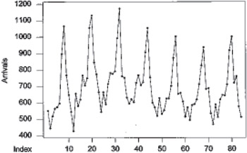
Figure 1: Time series plot for arrival of U.S. citizens for foreign travel (1971-1977)

Figure 1 clearly shows a seasonal pattern with a period of 12. It does not contain an obvious trend. The autocorrelation coefficients of the series are shown in Table 3.

Table 3: Autocorrelation coefficients of arrival series

Lag(k)	1	2	3	4	5	6	7	8	9	10	11	12	13	14	15	16	17	18	19
p(k)	0.617	0.233	-0.02	-0.28	-0.363	-0.4	-0.318	-0.209	0.027	0.224	0.506	0.745	0.435	0.12	-0.097	-0.303	0.393	-0.423	-0.189

The first six years of the data are used for estimating parameters in individual models. The five models described in section 3 are used. For the data, we generate one-step ahead forecast values for the last 12 periods using the five different individual forecasting methods. Therefore in each period we have five different forecast values. Based on these five forecast values in each period we can obtain a various combination forecast value such as the simple average forecast. However, we now propose to use the Bayesian approach and the Markov chain Monte Carlo method to generate the predictive values given the five forecast values from different individual time series models. Thus at the end we will obtain the empirical posterior predictive density which converges to the true distribution as the number of generated sample increases. The mode of the empirical posterior predictive distribution can be approximated by using the formula given in (19). So in each period we obtain a mode forecast. Lastly, the results are compared to the other combination methods, the simple average and the G1 and G2 methods.

Probability Intervals Using the MCMC Method

For each parameter, we have a MCMC sample from the posterior distribution of that parameter. A 100(1 - α)% probability interval for a parameter may be estimated by taking any range which contains 100(1 - α)% of the MCMC sample. Usually, we take the 100 α/2% and 100(1 - α/2)% quantiles of the sample, as the endpoints of the interval. In Table 5, we present 95% probability intervals calculated in this way. The probability interval should have a 95% chance to contain the true value.

Empirical Results

The final results from our Gibbs sampler scheme for the time series data are presented in Tables 4 and 5 together with forecast values from the other five methods.

Table 4: Results of individual forecast method

Forecast Period	Forecast by Box-Jenkin Method	Forecast by Winter's Method	Forecast by Decomp. Method	Forecast by Direct Smoothing Method	Forecast by State-Space Method
1	550.5	555.3	565.9	549.2	556.46
2	488.4	497.5	513.2	552.3	502.2
3	575.7	586.7	588.4	551.1	585.9
4	623.1	650.1	676.2	676.1	647.1
5	641.4	658.1	630.3	637.1	636.4
6	718.3	713.9	685.9	662.1	703.3
7	860.7	877.5	917.9	936.7	892.3
8	1012.0	1037.5	1051.5	987.7	1047.1
9	713.4	742.8	691.6	756.1	712.5
10	695.4	708.6	663.2	634.2	672.8
11	613.4	625.9	649.2	570.9	600.3
12	525.5	536.1	482.4	508.5	523.8

Table 5: Results of combination forecast methods

Forecast Period	Actual Value	Simple Average Method	G1 Method	G2 Method	Mode Forecast Method	Probability Interval
1	588.0	555.5	556.2	556.3	575.2	(504.6, 602.2)
2	511.0	510.7	498.2	498.2	522.7	(412.4, 573.8)
3	618.0	577.6	583.1	583.1	587.0	(517.3, 607.8)
4	645.0	654.5	647.1	646.9	665.6	(583.8, 696.3)
5	643.0	640.7	645.2	645.1	644.9	(559.1, 683.1)
6	710.0	696.7	708.1	708.2	701.9	(611.9, 731.3)
7	919.0	897.0	881.5	881.8	915.3	(797.5, 961.7)
8	1002.0	1027.2	1036.0	1034.2	1033.3	(929.5, 1084.4)
9	719.0	723.3	717.8	718.1	738.5	(605.9, 779.2)
10	760.0	674.9	689.6	690.0	690.3	(569.7, 747.7)
11	575.0	611.9	627.4	628.7	624.2	(510.8, 673.6)
12	511.0	515.3	520.3	519.2	518.8	(452.1, 547.3)

In Table 6 we show the RMSE values given by the individual forecasting methods as well as by the combination forecasting methods

Table 6: RMSE values of all the forecasting methods

	Forecast Method	RMSE Value
1	Box-Jenkin Method	33.7118
2	Winter's Method	31.4972
3	Decomp. Method	42.7940
4	Direct Smoothing Method	48.9200
5	State-Space Method	33.4001
6	Simple Average Method	32.5584
7	G1 Method	32.6062
8	G2 Method	32.4941
9	Posterior Mode Method	29.5342[a]
[a]: This indicates the minimum value.

The mode estimate has the least RMSE values. To strengthen our claim that the data followed a Weibull distribution, we use a Weibull probability plot for the 12 actual values in the forecasting period. The probability plot showed that all the data fall inside the 95% confidence interval and the Anderson-Darling test statistic value is equal to 1.34, which indicated a good fit.

---