Organizing Worksheets for Easy Reading | Online Traning Solutions

Before we discuss other calculations you might want to perform with this worksheet, let s look at ways to organize your information to make the results of calculations stand out from the data. As your worksheets grow in complexity, you ll find that paying attention to such details will keep you oriented and help others understand your results.

Usually when you create a worksheet, you are interested not so much in the individual pieces of information as in the results of the calculations you perform on the pieces. The current worksheet isn t very large, but often worksheets include many screens of information. It s a good idea to design your worksheets so that the important information is easily accessible and in a predictable location. For these reasons, we suggest that you leave room in the upper-left corner of your worksheets for a calculation area.

Calculation area advantages

Creating a calculation area at the top of your worksheet is a good habit to get into and offers the following advantages:

You don t have to scroll around looking for totals and other results.
You can print just the first page of a worksheet to get a report of the most pertinent information.
You can easily jump to the calculation area from anywhere on the worksheet by pressing Ctrl+Home to move to cell A1.

Setting Up a Calculation Area

To see first hand how helpful a calculation area can be, let s create an area at the top of Sheet1 of the 2002 Jobs workbook for a title and a set of calculations. You ll start by freeing up some space at the top of the worksheet:

Select A1:D16.
If necessary, drag the Formatting toolbar s move handle to the right until the Cut button joins the Copy and Paste buttons on the Standard toolbar. Then click the Cut button.
Select A10 , and click the Paste button.

Excel moves the selection to A10:D25, leaving room for a title.
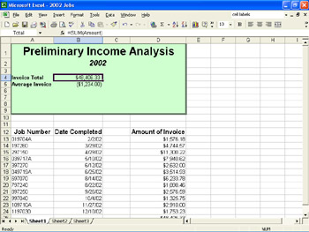
In cell A1 , type Preliminary Income Analysis , and click the Enter button.
Format the title by clicking the Bold button on the Formatting toolbar. Then click 10 in the Font Size box, type 22 , and press Enter .

The height of row 1 increases to accommodate the larger font.
In cell A2 , type 2002 , and click the Enter button.
Format the subtitle by clicking Ctrl+B and then Ctrl+I.

These keyboard shortcuts apply bold formatting and italic formatting, respectively.
Change the subtitle s font size to 14 , and press Enter .
Center the title above the calculation area by selecting A1:D1 and clicking the Merge and Center button on the Formatting toolbar s Toolbar Options palette.

Excel merges the four cells and centers the title over the selected area, but the title is still stored in cell A1.
Repeat step 9 for the subtitle, using the range A2:D2.

Now we re ready to set up the calculation area. With Excel, you can get really fancy, using borders and color to draw attention to calculation results.
Select A1:D9, and click Cells on the Format menu.
In the Format Cells dialog box, click the Border tab.
In the Line area, click the last option (the double line) in the second column of the Style box, and then click Outline in the Presets area.
Click the Patterns tab, select a light color from the palette, and click OK .

We left our calculation area white to make our graphics more legible. Excel surrounds the calculation area with a border and fills it with the color you selected. Now let s move the calculation in cell A10.
Click cell A4 , type Invoice Total, and press Enter .
Click cell A10 , and use the Cut and Paste buttons to move the formula to cell B4 .

We ll show you how to quickly restore the color to cell B4 in a moment.
Select A4:A9, and click the Bold button.
Click cell A5 , type Average Invoice , and click the Enter button.

The new heading is bold because you already applied the bold format to the range A4:A9. You can also apply number formats to empty cells to save time, as we ll see in a moment.
If necessary, click Column and then AutoFit Selection on the Format menu.

Excel widens column A so that the headings fit within the column. From now on, adjust the column width as necessary to see your work.
Select B4:B9, and click Cells on the Format menu.
Click the Number tab, click Currency in the Category list, and select the third option in the Negative numbers list. Be sure the Decimal Places setting is 2 , and then click OK .

Excel formats the selected cells with a dollar sign, a comma, and two decimal places.
To see the Currency format for negative numbers, click cell B5 , type -1234, and click the Enter button.

Excel displays the negative value in parentheses, aligning the value itself with the positive value above it.
To restore the background color to cell B4, make sure cell B5 is selected, click the Format Painter button on the Standard toolbar, and click cell B4 to duplicate the formatting of B5 in B4.

The results are shown in this graphic:

Displayed values vs. underlying values

After you apply a format, the value displayed in the cell might look different from the value displayed in the formula bar. For example, a value of 345.6789 is displayed in its cell as $345.68 after you apply the Currency format. When performing calculations, Excel uses the value in the formula bar, not the value displayed in the cell.