Overview of System Performance | Mastering BEA WebLogic Server: Best Practices for Building and Deploying J2EE Applications

In this section, we discuss the core principles and tuning techniques that underlie many of the performance best practices and troubleshooting tips that we cover later in the chapter. Having a good understanding of the basic operating system, network, JVM, and server resources and tuning options will help you apply these best practices and tips. It is not enough to know what to do; you need to understand why it helps.

Reviewing the Core Principles

Before we get started talking about techniques for achieving scalability , we should define the term itself. Scalability generally refers to the ability of an application to meet additional capacity demands without significantly affecting the request processing time. The term is also used to describe the ability to increase the capacity of an application proportional to the hardware resources added. For example, if the maximum capacity of an application running on four CPUs is 200 requests per second with an average of 1-second response time, then you might expect that the capacity for the application running on eight CPUs to be 400 requests per second with the same 1-second response time. This type of linear scalability is typically very difficult to achieve, but scalable applications should be able to approach linear scalability if the application s environment is properly designed. Good scalability in multi-tier architectures requires good end-to-end performance and scalability of each component in each tier of the application.

When designing enterprise-scale applications, you must first understand the application itself and how your users interact with it. You must identify all of the system components and understand their interactions. The application itself is a critical component that affects the scalability of the system. Understanding the distribution of the workload across the various tiers will help you understand the components affected most severely by user activity. Some systems will be database intensive ; others will spend a majority of their processing time in the application server. Once you identify these heavily used components, commonly referred to as application hotspots , you can use proper scaling techniques to prevent bottlenecks.

This strong understanding of the system itself will also allow you to choose the correct system architecture to meet the demands of the application. Once you choose the system architecture, you can begin to concentrate on the application and apply good performance design practices. There are no silver bullets for choosing the correct system architecture. In our experience, it is best to take an overall system approach to ensure that you cover all facets of the environment in which the application runs. The overall system approach begins with the external environment and continues drilling down into all parts of the system and application. Taking a broad approach and tuning the overall environment ensures that the application will perform well and that system performance can meet all of your requirements.

Note

WebLogic Server-based application performance depends on many different factors that include the network, operating system, application server, database, and application design and configuration. Many of these factors vary from installation to installation, so you should review all recommendations made in this chapter to determine if they are applicable to your environment.

Before we dive into the lower-level tuning techniques, let s review some system-level approaches for increasing the performance and throughput of your J2EE application.

Use more powerful machines. This technique applies equally well across the Web, application, and database tiers. If a particular tier s processing is CPU-intensive, then using more powerful machines can allow this layer to do the same amount of work in less time and/or to do more work, thereby increasing throughput. Keep in mind that this technique is effective only on CPU-intensive applications. If your system performance is limited by I/O operations, adding processing power will do very little to improve performance or eliminate bottlenecks. Increasing an application s capacity by adding more CPUs to a machine is often referred to as vertical scaling .

Use clustering. By distributing the load across multiple Web and/or application servers, you can increase the capacity of your application. Increasing an application s capacity by adding more machines is often referred to as horizontal scaling . Horizontal scaling also provides a secondary benefit: increased redundancy at the hardware level to improve the overall system reliability.

Take advantage of network appliances. Today, there are a wide variety of specialized hardware devices that are optimized to perform specific tasks , such as fast and reliable data storage, content caching, load balancing, and SSL termination. These devices operate at various layers within the system architecture and can either offload or significantly reduce the processing work that the software needs to do, and do it in a much more scalable way than can be accomplished with software only. As such, they can dramatically increase the performance and scalability of your applications.

Cache whenever possible. Caching can significantly improve response time and increase the scalability of Web, application, and database servers. Network appliances that cache static content and prevent those requests from ever hitting the Web servers can dramatically improve performance. Most Web servers also offer page caching, which you should use whenever possible. WebLogic Server also offers dynamic content caching through its JSP caching features, a technique discussed in Chapter 1. WebLogic Server 8.1 adds support for RowSets in addition to its various options for entity bean caching; you can use these to cache application data to reduce trips to the database or other back-end systems. Of course, caching application data that changes frequently can often create more problems than it solves . In most cases, we recommend using the database to cache this data. Most database management systems offer a variety of tuning options for optimizing their caching strategies to better suit a particular application; this can significantly reduce the amount of I/O that the database has to do to answer application queries. You should evaluate each of these techniques to determine how best to use caching to improve your application s performance and scalability.

Tuning a WebLogic Server-Based Application

Achieving maximum performance and scalability for your WebLogic Server-based application requires tuning at many different layers within the overall environment. We ll structure our discussion of tuning from the bottom-up, starting with the operating system itself and ending with application-server tuning.

Operating System Tuning

Many J2EE applications have some sort of Web interface through which the users interact. HTTP is a stateless protocol used by browsers to talk to Web and/or application servers. When initiating a request, the browser opens a connection to the server, sends a request, waits for the response, and then closes the connection. Although HTTP keep- alive allows the browser to reuse an existing connection to the server for multiple requests, both the browser and the server will typically close the connection after a fairly short period of inactivity. A typical time-out for one of these connections might be 30 seconds or less. As a result, busy Web applications with hundreds, or even thousands, of concurrent users will open and close a large number of connections between the browser and the Web or application server.

These HTTP connections to the Web or application server are nothing more than operating system-level TCP sockets. All modern operating systems treat sockets as a specialized form of file access and use data structures called file descriptors to track open sockets and files for an operating system process. To control resource usage for processes on the machine, the operating system restricts the number of open file descriptors per process. The default number of file descriptors available for a process depends on the operating system type and its configuration. Without going too far into the gory details of TCP/IP, you should be aware that all TCP connections that have been gracefully closed by an application will go into what is known as the TIME_WAIT state before being discarded by the operating system. The length of time that the socket stays in the TIME_WAIT state is commonly known as the time wait interval . While in this TIME_WAIT state, the operating system will maintain the resources allocated for the socket, including its file descriptor. To learn more about the details of this, see Internetworking with TCP/IP Volume II: Design, Implementation, and Internals by Douglas A. Comer and David L. Stevens (Prentice Hall, 1998).

As a result of this phenomenon , combined with the fact that HTTP servers end up opening and closing a lot of TCP sockets, busy server processes can fill up the server process s file descriptor table. To deal with this problem, you often need to tune the operating system to allow your application to scale without running into these operating system limits. When tuning the operating system, you should follow your hardware vendor s tuning recommendations, if these exist. Remember to tune the operating system on all machines that exist in the system, especially any Web or application server machines that use the HTTP protocol. On Unix servers, this typically means tuning the number of file descriptors and/or some of the TCP/IP device driver s tuning parameters. On platforms such as HP-UX, it may be necessary to change some of the kernel parameters. When tuning TCP parameters, you should work with your system administrator to determine what modifications your machines require.

Each operating system sets important tuning parameters differently. We will start with a detailed coverage of the Solaris operating system and then briefly discuss the differences on other common Unix operating systems and Windows .

Tuning Solaris

On Solaris, one common problem is that the default value for the time wait interval is too high for high-volume HTTP servers. On most Unix operating systems, you can determine the number of sockets in the TIME_WAIT state using the netstat command:

 netstat a  grep TIME_WAIT  wc l

This command will count all of the TCP connections that are in the TIME_WAIT state. As this number approaches the maximum number of file descriptors per process, your application s throughput will suffer dramatic degradations because new connection requests may have to wait for a free space in the application s file descriptor table. To determine the current setting for the time wait interval, use the ndd command shown here:

 /usr/sbin/ndd /dev/tcp tcp_time_wait_interval

Note that prior to Solaris 2.7, this parameter was somewhat erroneously called tcp_close_wait_interval . By default, Solaris sets this parameter to 240,000 milliseconds, or 4 minutes. Our recommendation, which follows the recommendations of both BEA and SUN, is to reduce this setting to 60,000 milliseconds , or 1 minute. You should use the following ndd command to change the tcp_time_wait_interval setting dynamically:

 /usr/sbin/ndd -set /dev/tcp tcp_time_wait_interval 60000

This command will change the setting of the TCP device driver for the entire machine and therefore requires superuser privileges. Be forewarned that this value, and any other values you change with ndd , will reset to the default value when you reboot the machine. To make the changes permanent, you will need to create a boot script.

According to recommendations on Sun s Web site at http://docs.sun.com/db/doc/816-0607/6m735r5fl?a=view, you want the ndd boot script to run between the S69inet and S72inetsvc scripts. This means that you should create the script file in the /etc/init.d directory and create symbolic links to your script from the /etc/rc2.d , /etc/rc1.d , and /etc/rcS.d directories. The link names should begin with either S70 or S71 because the S tells Solaris that this script should run at startup and the numeric value determines the order in which the scripts run.

There are a number of other TCP- related parameters available on Solaris that may yield performance improvements in certain situations. To get a list of all of the names of the TCP device driver parameters, use the following ndd command:

 ndd /dev/tcp \?

The output from this command will also show you which parameters are read-write and which ones are read-only . Read-only parameters cannot be changed with ndd and must be changed in /etc/system . In addition to the tcp_time_wait_interval parameter, you may also want to consider changing some of the other parameters like tcp_conn_hash_size , tcp_conn_req_max_q , tcp_xmit_hiwat , and tcp_recv_hiwat parameters.

The tcp_conn_hash_size parameter controls the size of a hash table that helps quickly locate the TCP socket s data structure in the kernel. If the size is too small, it will result in long hash chains in each bucket that force the operating system into a linear search for the socket entry of interest, and performance will suffer accordingly . By default, Solaris 8 and 9 set this parameter to 512; we recommend raising the value to 8192 for machines hosting HTTP servers. To set tcp_conn_hash_size , change the /etc/system file, as shown here:

 set tcp:tcp_conn_hash_size=8192

The tcp_conn_req_max_q parameter controls the maximum allowable number of completed connections waiting to return from an accept call (that have completed the three-way TCP connection handshake). You should increase this parameter only if you notice that your system is dropping connections. You can determine the number of drops using the netstat command:

 netstat s  grep tcpListenDrop

By default, this value is set to 128. If the system is dropping connections, try increasing the value of tcp_conn_req_max_q to 1024.

The tcp_xmit_hiwat and tcp_recv_hiwat parameters control the default size of the send window and receive window for each TCP connection, respectively. On very fast networks, you should make sure that the values are set to at least 32K. By default, Solaris 8 sets these parameters to 16K and 24K, respectively. Solaris 9 changes the default settings for both parameters to 48K.

Best Practice

Increase the size of key TCP-related parameters to improve system performance and reduce dropped connections.

As we mentioned previously, most operating systems limit the number of open file descriptors a process can have. On Solaris (and most other Unix operating systems), there are actually two file descriptor limits. The first limit is the default limit imposed on each process; this is sometimes called the soft limit. The second limit is the maximum number of file descriptors per process that the operating system can support in its current configuration; this is sometimes called the hard limit. Use the ulimit command to change the soft limit to increase the maximum number of file descriptors for a particular process. You can increase this number only up to the hard limit unless you are the superuser , whose username is typically root ”regardless of any feedback that the ulimit command may give you to the contrary. To change the hard limit for processes not running as the root user, you need to reconfigure the operating system. On Solaris, this means modifying the /etc/system file. The two parameters of interest in the /etc/system file are rlim_fd_cur and rlim_fd_max , which control the soft and hard limits, respectively. You will need to reboot the machine in order for changes to the /etc/system file to take effect.

For any machine that will host an HTTP server, we strongly recommend that you increase both the soft and hard limits to 4096 or even 8192. Please make sure to check your operating system documentation and release notes; there are some negative performance implications on some older versions of Solaris if you set these numbers too high. The syntax for adjusting these parameters in the /etc/system file is shown here:

 set rlim_fd_cur=4096 set rlim_fd_max=4096

Best Practice

On any machine that hosts an HTTP server, increase the maximum number of file descriptors per process to either 4096 or 8192. On Solaris, this means setting the rlim_fd_cur and rlim_fd_max parameters in the /etc/system file and rebooting the machine.

For more information on tuning the Solaris operating system, please refer to the Solaris Tunable Parameters Reference Manual , available on Sun s Web site at http://docs.sun.com/db/doc/816-0607 (Solaris 8) or http://docs.sun.com/db/doc/806-7009 (Solaris 9).

Tuning AIX

On AIX, the no command is equivalent to the ndd command on Solaris. Running the no “a command will display the current values of all network attributes. Issuing the following command will change the time wait interval:

 no o tcp_timewait=4

This example command sets the tcp_timewait parameter to 4 15-second intervals, or 1 minute. For more information on the no command, see http://publib16.boulder.ibm.com/pseries/en_US/cmds/aixcmds4/no.htm .

When a server listens on a port for connections, TCP creates a queue that it uses to buffer connection requests while waiting for the server to accept the connection. This listen queue is a fixed size, and if it fills up, the operating system will reject any new connection requests until there is space available in the queue. AIX controls the maximum length of this listen queue with the somaxconn parameter. By default, AIX sets this to 1024, but on machines with busy HTTP servers, you might want to increase this to 8192. Note that this increases only the maximum allowable length of the listen queue. You will still need to adjust the WebLogic Server instance s Accept Backlog parameter so that WebLogic Server will ask for a longer listen queue, using the server s Tuning Configuration tab in the WebLogic Console. Of course, this particular configuration is also important for other operating systems, including Solaris.

Some other TCP parameters you may need to tune on AIX include tcp_sendspace and tcp_recvspace , which control the socket s sending and receiving buffer sizes, respectively. For more information about tuning AIX, please refer to the AIX Performance Management Guide at http://publib16.boulder.ibm.com/pseries/en_US/aixbman/prftungd/prftungd.htm .

Tuning HP-UX

HP-UX provides the ndd command to use for setting the TCP parameters, just like Solaris (although parameter names are slightly different). To adjust the maximum allowable length of the listen queue to 1024, execute the ndd command shown here:

 ndd set /dev/tcp tcp_conn_req_max 1024

By default, HP-UX sets the tcp_time_wait_interval to 60000 milliseconds, so you do not typically need to adjust this. HP-UX reads a file in /etc/rc.config.d/nddconf to get customized settings for the TCP parameters at boot time. See this file for further information about how to use it to customize the TCP settings for your machine.

On HP-UX, you may also need to modify some kernel parameters to ensure that WebLogic Server performs optimally. Use the /usr/sbin/sam program to modify kernel parameters. HP-UX limits the maximum number of threads per process. On older versions of HP-UX, this value defaults to 64, a value that large applications can easily exceed. Newer versions of HP-UX set the default value to 256, but you can change this using the max_thread_proc kernel parameter. The maximum number of threads allowed on the system at any point in time is set using the nkthread kernel parameter. Older versions of HP-UX come with a default value of 499 that can be too low on larger multi-CPU machines; newer versions have a default value of 8416. Also remember to adjust the maxfile and maxfile_lim parameters that control the soft and hard limits on the maximum number of file descriptors, if needed. For more information on kernel tuning parameters, see http://docs.hp.com/hpux/onlinedocs/TKP-90203/TKP-90203.html .

Tuning Linux

When tuning Linux operating systems, use either the sysctl command or the /proc file system. Because the sysctl command provides the ability to read from the /etc/sysctl.conf file, we generally prefer to use sysctl over the /proc method. On Linux, the default time wait interval is 120 seconds; you can reset this by changing the value of the ip_ct_tcp_timeout_time_wait parameter:

 sysctl -w ip_ct_tcp_timeout_time_wait=60

Linux also limits the maximum number of open files for all users. If this is set too low, your HTTP server process might run out of file descriptors. To change this setting, you can add an entry into the /etc/sysctl.conf file and then run sysctl “p . The required entry is

 fs.file-max = 20000

Then, if you want to allow your HTTP server process to be able to have 8,192 open file descriptors, you need to edit the /etc/security/limits.conf file to add the following entry for your weblogic user ( assuming that the server is running as user weblogic ). Remember that this number applies across all processes running as the weblogic user. The entry is

 weblogic hard nofile 8192

Finally, you need to use the ulimit command to actually make the setting active for the current login session, as shown here:

 ulimit n 8192

For more information on Linux tuning, please consult you Linux vendor s documentation or check out some of the Linux resources on the Web, such as http://ipsysctl-tutorial.frozentux.net/ipsysctl-tutorial.html , which provides a description of the TCP/IP tuning parameters available on Linux.

Tuning Windows

The concepts behind tuning the Windows operating system are similar to those for tuning other operating systems. Most of the TCP/IP parameter settings are located in the registry under the HKEY_LOCAL_MACHINE\SYSTEM\CurrentControlSet\Services folder. To change the maximum length of the TCP listen queue, whose default value is 15, you create a DWORD entry called ListenBackLog in the Inetinfo\Parameters subfolder in your Windows registry. Windows sets the default for the time wait interval to four minutes; the TcpTimedWaitDelay parameter in the Tcpip\Parameters subfolder allows you to change its value. For more information on tuning Windows, please consult the Microsoft Windows documentation. One excellent paper that discusses the Microsoft TCP/IP implementation in Windows 2000 can be found at http://www.microsoft.com/windows2000/techinfo/howitworks/communications/networkbasics/tcpip_implement.asp .

Network Tuning

Most networks today are very fast and are rarely the direct cause of performance problems in well-designed applications. In our experience, the most frequent network problems come from misconfigured network devices. Whether it is a network interface card in your server, a firewall, a router, or another, more specialized network device such as a load balancer, improper configuration can lead to insidious problems that are very difficult to figure out. This is why it is important to monitor your network when troubleshooting performance problems. Some very simple tests can indicate problems with the network.

First, you can use the ping command to generate network traffic between two nodes in your network and look for packet loss. On a high-speed local area network, you should almost never see any packet loss. If you are only seeing performance problems during peak load, make sure to run your ping tests during these times to make sure that the network is still working properly under load. Second, look for send or receive errors on your machine s network interface. You can use the netstat command shown here to do this on Solaris:

 netstat I /dev/hme0 5

This command will generate output every five seconds that shows the statistics for the hme0 network interface card. Always remember that the first line of output is the cumulative output since the last reboot, so you should generally ignore it. The output of this command will look similar to that shown here. Pay particular attention to the errs columns .

 input   /dev/h    output           input  (Total)    output packets errs  packets errs  colls  packets errs  packets errs  colls 0       0     0       0     0      142034  0     40794   242   0 0       0     0       0     0      48      0     6       0     0 0       0     0       0     0      50      0     7       0     0 0       0     0       0     0      48      0     7       0     0

Even when the network is properly configured, it is still important to monitor your network performance in both your testing and production environments, concentrating on three areas: packet retransmissions, duplicate packets, and listen drops of packets.

Packet retransmissions occur when the TCP layer is not receiving acknowledgments (ACKs) from the receiver quickly enough, causing TCP to retransmit the packet. If your retransmission rate is 15 percent or higher, this generally indicates a problem with the network. Bad network hardware or a slow or congested route can cause excessive packet retransmission. You should monitor retransmissions using the netstat “s “P tcp command to get the tcpRetransBytes and tcpOutDataBytes statistics. From these numbers, calculate the retransmission percentage using the following formula:

If the remote system is retransmitting too quickly, this will cause duplicate packets. Like packet retransmissions, duplicate packets can also indicate a bad network device or a slow or congested route. Using the same netstat command we just showed you, get the tcpInDupBytes and tcpInDataBytes statistics and calculate the duplication percentage using the following formula:

Listen drops occur when your system has a full listen queue and cannot accept any new connections. To eliminate listen drops, increase the size of the Solaris TCP parameter tcp_conn_req_max_q (or its equivalent on your operating system) or add more servers to handle the network load. Use the netstat “s “P tcp grep tcpListenDrop command to measure the frequency of listen drops.

Best Practice

Modern networks are fast enough to avoid performance problems in well-designed systems, but you should monitor key network statistics such as packet retransmissions, duplicate packets, and listen drops to ensure good performance. When troubleshooting performance problems, don t forget to check your network for packet loss or errors.

Java Virtual Machine Tuning

The Java Virtual Machine (JVM) you use to run your WebLogic Server-based application is a key factor in the final server performance. Not all JVMs are created equal ”we have seen certain applications perform up to 20 percent better simply by using a different JVM. Performance is nothing without stability, and fast applications do not do your users any good if they are not running. We recommend that you look for stability first and then performance when selecting the JVM on which to run your application server. If more than one JVM is available and supported on your target deployment environment, you should test them head to head to determine which JVM best meets your reliability, performance, and scalability requirements.

Garbage collection is the single most important factor when tuning a JVM for long-running, server-side applications. Improperly tuned garbage collectors and/or applications that create unnecessarily large numbers of objects can significantly affect the efficiency of your application. It is not uncommon to find that garbage collection consumes a significant amount of the overall processing time in a server-side Java application. Proper tuning of the garbage collector can significantly reduce the garbage collector s processing time and, therefore, can significantly improve your application s throughput.

While we spend most of our time in the next sections specifically talking about the Sun JVM, a lot of these concepts are similar in other JVMs, such as BEA s JRockit. Our discussion of JVM tuning will start by reviewing garbage collection. Next , we will walk through key JVM tuning parameters and options for the SUN JVM. We will touch briefly on JRockit toward the end of this section.

Understanding Garbage Collection

Garbage collection (GC) is the technique a JVM uses to free memory occupied by objects that are no longer being used by the application. The Java Language Specification does not require a JVM to have a garbage collector, nor does it specify how a garbage collector should work. Nevertheless, all of the commonly used JVMs have garbage collectors, and most garbage collectors use similar algorithms to manage their memory and perform collection operations.

Just as it is important to understand the workload of your application to tune your overall system properly, it is also important to understand how your JVM performs garbage collection so that you can tune it. Once you have a solid understanding of garbage collection algorithms and implementations , it is possible to tune application and garbage collection behavior to maximize performance. Some garbage collection schemes are more appropriate for applications with specific requirements. For example, near-real-time applications care more about avoiding garbage collection pauses while most OLTP applications care more about overall throughput. Once you have an understanding of the workload of the application and the different garbage collection algorithms your JVM supports, then you can optimize the garbage collector configuration.

In this section, we give you a brief overview of different approaches that JVMs use for garbage collection. For more information on garbage collection algorithms and how they affect JVM performance, we recommend looking at the two very good articles on Sun s Web site: Improving Java Application Performance and Scalability by Reducing Garbage Collection Times and Sizing Memory by Nagendra Nagarajayya and Steve Mayer (http://wireless.java.sun.com/midp/articles/garbage) and Improving Java Application Performance and Scalability by Reducing Garbage Collection Times and Sizing Memory Using JDK 1.4.1 - New Parallel and Concurrent Collectors for Low Pause and Throughput applications by Nagendra Nagarajayya and Steve Mayer, (http://wireless.java.sun.com/midp/articles/garbagecollection2).

As we discussed previously, the purpose of the garbage collection in a JVM is to clean up objects that are no longer being used. Garbage collectors determine whether an object is eligible for collection by determining whether objects are being referenced by any active objects in the system. The garbage collector must first identify the objects eligible for collection. The two general approaches for this are reference counting and object reference traversal. Reference counting involves storing a count of all of the references to a particular object. This means that the JVM must properly increment and decrement the reference count as the application creates references and as the references go out of scope. When an object s reference count goes to zero, it is eligible for garbage collection.

Although early JVMs used reference counting, most modern JVMs use object reference traversal. Object reference traversal simply starts with a set of root objects and follows every link recursively through the entire object graph to determine the set of reachable objects. Any object that is not reachable from at least one of these root objects is garbage collected. During this object traversal stage, the garbage collector must remember which objects are reachable so that it can remove those that are not; this is known as marking the object.

The next thing that the garbage collector must do is remove the non-reachable objects. When doing this, some garbage collectors simply scan through the heap, removing the unmarked objects and adding their memory location and size to a list of available memory for the JVM to use in creating new objects; this is commonly referred to as sweeping . The problem with this approach is that memory can fragment over time to the point where there are a lot of small segments of memory that are not big enough to use for new objects but yet, when added all together, can make up a significant amount of memory. Therefore, many garbage collectors actually rearrange live objects in memory to compact the live objects, making the available heap space contiguous.

In order to do their jobs, garbage collectors usually have to stop all other activity for some portion of the garbage collection process. This stop-the-world approach means all application-related work stops while the garbage collector runs. As a result, any in-flight requests will experience an increase in their response time by the amount of time taken by the garbage collector. Other, more sophisticated collectors run either incrementally or truly concurrently to reduce or eliminate the application pauses. Some garbage collectors use a single thread to do their work; others employ multiple threads to increase their efficiency on multi-CPU machines. Let s look at a few of the garbage collectors used by modern JVMs.

Mark-and-sweep collector. This type of collector first traverses the object graph and marks reachable objects. It then scans the heap for unmarked objects and adds their memory to a list of available memory segments. This collector typically uses a single thread to do its work and is a stop-the-world collector.

Mark-and-compact collector. A mark-and-compact collector, sometimes known as a mark-sweep-compact collector, uses the same marking phase as a mark-and-sweep collector. During the second phase, it compacts the heap by copying marked objects to a new area of the heap. These collectors are also stop-the-world collectors.

Copying collector. This type of collector divides the heap into two areas, commonly known as semi-spaces . It uses only one semi-space at a time; the JVM creates all new objects in one semi-space. When the garbage collector runs, it copies any reachable objects it finds to the other semi-space as it finds them, thus compacting the heap as it copies live objects. All dead objects are left behind. This algorithm works well for short-lived objects, but the expense of continually copying long-lived objects makes it less efficient. Again, this is a stop-the-world collector.

Incremental collector. Incremental collectors basically divide the heap into multiple areas and collect garbage from only one area at a time. This can create much smaller, though more frequent, pauses in your application. There are numerous approaches defining how the actual collection is handled from traditional mark-and-sweep to algorithms designed explicitly for use with multiple smaller areas like the train algorithm. See Incremental Mature Garbage Collection Using the Train Algorithm by Jacob Seligmann and Steffen Grarup (http://www.daimi.aau.dk/~beta/Papers/Train/train.html) for more information.

Generational collector. This type of collector divides the heap into two or more areas that it uses to store objects with different lifetimes. The JVM generally creates all new objects in one of these areas. Over time, the objects that continue to exist get tenure and move into another area for longer-lived objects. Generational collectors often use different algorithms for the different areas to optimize performance.

Concurrent collectors. Concurrent collectors run concurrently with the application, typically as one or more background threads. These collectors typically have to stop-the-world at some point to complete certain tasks, but the amount of time they halt all processing is significantly reduced because of their other background work.

Parallel collectors. Parallel collectors typically use one of the traditional algorithms but use multiple threads to parallelize their work on multiprocessor machines. Using multiple threads on multi-CPU machines can dramatically improve the scalability of a Java application on multiprocessor machines.

Tuning the Sun HotSpot 1.4.1 JVM Heap Size

Sun Microsystem s HotSpot JVM uses a generational collector that partitions the heap into three main areas: the new generation area, the old generation area, and the permanent generation area. The JVM creates all new objects in the new generation area. Once an object survives a certain number of garbage collection cycles in the new generation area, it gets promoted, or tenured , to the old generation area. The JVM stores Class and Method objects for the classes it loads in a section of the heap known as the permanent generation area. From a configuration perspective, the permanent generation area in the Sun HotSpot 1.4.1 JVM is a separate area that is not considered part of the heap. Before we go any further, let s look at how to control the size of these areas.

You can use the -Xms and -Xmx flags to control the initial and maximum size of the entire heap, respectively. For example, the following command sets the initial size of the entire heap to 128 megabytes (MBs) and the maximum size to 256 MBs:

 java -Xms128m -Xmx256m ...

To control the size of the new generation area, you can use the -XX:NewRatio flag to set the proportion of the overall heap that is set aside for the new generation area. For example, the following command sets the overall heap size to 128 MBs and sets the new ratio to 3. This means that the ratio of the new area to the old area is 1:3; the new area is one-fourth of the overall heap space, or 32 MBs, and the old area is three-fourths of the overall heap space, or 96 MBs.

 java -Xms128m -Xmx128m -XX:NewRatio=3 ...

The initial and maximum sizes for the new area can be set explicitly using the -XX:NewSize and -XX:MaxNewSize flags or the new Java 2 SDK 1.4 -Xmn flag. For example, the command shown here sets the initial and maximum size to 64 MBs:

 java -Xms256m -Xmx256m -Xmn64m ...

Configuration-wise, the permanent area is not considered part of the heap. By default, the initial size of the permanent area is 4 MBs. As your application loads and runs, the JVM will resize the permanent area as needed up to the maximum size for this area. Every time it resizes the permanent area, the JVM does a full garbage collection of the entire heap (and the permanent area). By default, the maximum size is 32 MBs. Use the -XX:MaxPermSize flag to increase the maximum size of the permanent area. When loading large numbers of classes in your WebLogic Server application, it is not uncommon to need to increase the maximum size of this area. The number of objects stored in the permanent area will grow quickly while the JVM loads classes, and it may force the JVM to resize the permanent area frequently. To prevent this resizing, set the initial size of the permanent area using the -XX:PermSize flag. For example, here we have set the initial size to 32 MBs and the maximum size to 64 MBs:

 java -Xms512m -Xmx512m -Xmn128m -XX:PermSize=32m -XX:MaxPermSize=64m ...

Warning

When the permanent area of the heap is too small, the JVM will do a full garbage collection of the entire heap before resizing the permanent area. If you allow the JVM to control the size, these full garbage collections will happen relatively frequently because the JVM is ultra -conservative about grabbing too much space for the permanent area. Always set the PermSize big enough for your application to run comfortably.

By default, HotSpot uses a copying collector for the new generation area. This area is actually subdivided into three partitions. The first partition, known as Eden , is where all new objects get created. The other two semi-spaces are also called survivor spaces. When Eden fills up, the collector stops the application and copies all reachable objects into the current from survivor space. As the current from survivor space fills up, the collector will copy the reachable objects to the current to survivor space. At that point, the from and to survivor spaces switch roles so that the current to space becomes the new from space and vice versa. Objects that continue to live are copied between survivor spaces until they achieve tenure, at which point they are moved into the old generation area.

Use the “XX:SurvivorRatio flag to control the size of these subpartitions. Like the NewRatio , the SurvivorRatio specifies the ratio of the size of one of the survivor spaces to the Eden space. For example, the following command sets the new area size to 64 MBs, Eden to 32 MBs, and each of the two survivor spaces to 16 MBs:

 java -Xms256m -Xmx256m -Xmn64m -XX:SurvivorRatio=2 ...

Figure 12.1 shows an overview of the HotSpot JVM heap layout and some of the parameters that we have been discussing.

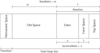
Figure 12.1: Understanding the HotSpot heap partitioning.

As we discuss previously, HotSpot defaults to using a copying collector for the new area and a mark-sweep-compact collector for the old area. Using a copying collector for the new area makes sense because the majority of objects created by an application are short-lived. In an ideal situation, all transient objects would be collected before making it out of the Eden space. If we were able to achieve this, and all objects that made it out of the Eden space were long-lived objects, then ideally we would immediately tenure them into the old space to avoid copying them back and forth in the survivor spaces.

Unfortunately, applications do not necessarily fit cleanly into this ideal model as they tend also to have a small number of intermediate-lived objects. It is typically better to keep these intermediate-lived objects in the new area because copying a small number of objects is generally less expensive than compacting the old heap when they have to be garbage collected in the old heap.

To control the copying of objects in the new area, use the -XX:TargetSurvivorRatio flag to control the desired survivor space occupancy after a collection. Don t be misled by the name ; this value is a percentage. By default, the value is set to 50. When using large heaps in conjunction with a low SurvivorRatio , you should probably increase this value to somewhere in the neighborhood of 80 to 90 to better utilize the survivor space.

Use the -XX:MaxTenuringThreshold flag to control the upper threshold the copying collector uses before promoting an object. If you want to prevent all copying and automatically promote objects directly from Eden to the old area, set the value of MaxTenuringThreshold to 0. If you do this, you will in effect be skipping the use of the survivor spaces, so you will want to set the SurvivorRatio to a large number to maximize the size of the Eden area, as shown here:

 java ... -XX:MaxTenuringThreshold=0 -XX:SurvivorRatio=50000 ...

Now that you understand the goals and controls you have for tuning the heap sizes, let s look at some of the information you can get from the JVM to help you make the right tuning decisions.

The “verbose:gc switch gives you basic information about what the garbage collector is doing. By turning this switch on, you will get information about when major and minor collections occur, what the memory size before and after the collection was, and how much time the collection took. Let s look at some sample output from this switch:

 [Full GC 21924K->13258K(63936K), 0.3854772 secs] [GC 26432K->13984K(63936K), 0.0168988 secs] [GC 27168K->13763K(63936K), 0.0068799 secs] [GC 26937K->14196K(63936K), 0.0139437 secs]

The first line that starts with Full GC is a major collection of the entire heap. The other three lines are minor collections, either of the new or the old area. The numbers before the arrow indicate the size of the heap before the collection, while the number after the arrow shows the size after the collection. The number in parentheses is the total size of the heap, and the time values indicate the amount of time the collection took.

By turning on the -XX:+PrintGCDetails switch, you can get a little more information about what is happening in the garbage collector. Output from this switch looks like this:

 [Full GC [Tenured: 11904K->13228K(49152K), 0.4044939 secs]           21931K->13228K(63936K), 0.4047285 secs] [GC [DefNew: 13184K->473K(14784K), 0.0213737 secs]           36349K->23638K(63936K), 0.0215022 secs]

As with the standard garbage collection output, the Full GC label indicates a full collection. Tenured indicates that the mark-sweep-compact collector has run on the old generation; the old heap size went from 11904K to 13228K; the total old area size is 49152K. The reason for this increase is that the new area is automatically purged of all objects during a full collection. The second set of numbers associated with the first entry represents the before, after, and total size of the entire heap. This full collection took 0.4047285 seconds. In the second entry, the GC label indicates a partial collection, and DefNew means that the collection took place in the new area; all of the statistics have similar meanings to the first except that they pertain to the new area rather than the old area.

By adding the -XX:+PrintGCTimeStamps switch, the JVM adds information about when these garbage collection cycles occur. The time is measured in seconds since the JVM started, shown in bold here:

  21.8441  : [GC  21.8443  : [DefNew: 13183K->871K(14784K), 0.0203224 secs]                        20535K->8222K(63936K), 0.0205780 secs]

Finally, you can add the -XX:+PrintHeapAtGC switch to get even more detailed information. This information will dump a snapshot of the heap as a whole.

To get more information on what is going on in the new area, you can print the object tenuring statistics by adding the -XX:+PrintTenuringDistribution switch, in addition to the -verbose:gc switch, to the JVM command line. The output that follows shows objects being promoted through the ages on their way to being tenured to the old generation.

 java -Xms64m -Xmx64m -XX:NewRatio=3 -verbose:gc       -XX:+PrintTenuringDistribution ... [GC Desired survivor size 819200 bytes, new threshold 31 (max 31) - age   1:     285824 bytes,     285824 total  34956K->22048K(63936K), 0.2182682 secs] [GC Desired survivor size 819200 bytes, new threshold 31 (max 31) - age   1:     371520 bytes,     371520 total - age   2:     263472 bytes,     634992 total  35231K->22389K(63936K), 0.0413801 secs] [GC Desired survivor size 819200 bytes, new threshold 3 (max 31) - age   1:     436480 bytes,     436480 total - age   2:     203952 bytes,     640432 total - age   3:     263232 bytes,     903664 total  35573K->22652K(63936K), 0.0432329 secs]

Notice the desired survivor size of 819200 bytes. Why is that? Well, let s do the math. If the overall heap is 64 MBs and the NewRatio is 3, this means that the new area is one-fourth of the total heap, or 16 MBs. Because we are using the client JVM, the default value of the SurvivorRatio is 8. This means that each survivor space is one- eighth the size of the Eden space. Because there are two survivor spaces, that means that each survivor space is one-tenth of the overall new area size, or 1.6 MBs. Because the default TargetSurivorRatio is 50 percent, this causes the desired survivor size to be about 800 KBs.

You will also notice that the maximum threshold is always 31. Because of the TargetSurvivorRatio discussion previously, the garbage collector will always try to keep the survivor space at or below the target size. The garbage collector will try to age (copy) the objects up to the threshold of 31 times before promoting them into the old area. The garbage collector, however, will recalculate the actual threshold for promotion after each garbage collection. Remember, any full garbage collection cycle will immediately tenure all reachable objects, so always try to tune the garbage collector ”especially the PermSize ”to prevent full garbage collection cycles from occurring.

In the last entry, you will notice that the garbage collector changed the threshold from the default of 31 to 3. This happened because the garbage collector is attempting to keep the occupancy of the survivor space at its desired survivor size . By adding the size of the objects in all three age categories you will get 903661 bytes, which exceeds the desired survivor size; therefore, the garbage collector reset the threshold for the next garbage collection cycle.

Java 2 SDK 1.4.1 comes with several new garbage collectors that allow you to optimize the garbage collector based on your application requirements. Let s look at those now to understand the available collectors and what they can do for you.

Selecting the Garbage Collector

While the generational garbage collection makes the HotSpot JVM much more efficient, several problems remain . Both the copying collector and the mark-sweep-compact collector are stop-the-world collectors. Increasing the size of the heap that these collectors must manage means increasing the pause times, regardless of how much processing power the box has. The primary reason for this is that both collectors use a single thread to do their work and, therefore, cannot take advantage of multiprocessor machines. This severely limits their scalability on large Symmetric Multi-Processor (SMP) boxes.

Java 2 SDK 1.4.1 comes with three new garbage collectors: the parallel copying collector, the concurrent old area collector, and the parallel scavenger collector. The first two collectors are designed to minimize application pauses, while the last collector is designed to increase throughput for applications that can tolerate pauses.

The parallel copying collector works just like the copying collector except that it will use multiple threads, one per CPU by default, to do its work. To enable this collector, you can set the -XX:+useParNewGC switch. If the machine has only one CPU, the JVM will default to the copying collector because multiple CPUs are not available. You can force the JVM to use the parallel copying collector by increasing the degree of parallelism manually using the -XX:ParallelGCThreads option:

 java ... -XX:+UseParNewGC -XX:+ParallelGCThreads=4 ...

The parallel copying collector can work in conjunction with either the concurrent old area collector or the traditional mark-sweep-compact collector.

When doing its work, the concurrent old area collector collects garbage in six steps, four that run concurrently with the application threads and two that stop-the-world. This makes for much smaller application pauses while doing an old generation garbage collection cycle. To use this new collector, simply set the -XX:+UseConcMarkSweepGC switch. If the concurrent collector is not able to keep up, the default mark-sweep-compact collector will step in. By default, the concurrent collector kicks in when the occupied percentage goes above 68 percent. You can control this threshold percentage using the -XX:CMSInitiatingOccupancyFraction flag, as shown here:

 java ... -XX:+UseConcMarkSweepGC -XX:CMSInitiatingOccupancyFraction=40 ...

By combining this and the parallel copying collector, you can significantly reduce the garbage collection pauses in your application on a multiprocessor machine.

To maximize the throughput for applications that can tolerate pauses, use the parallel scavenger collector by specifying the -XX:+UseParallelGC switch. Currently, this collector works only in conjunction with the old area s mark-sweep-compact collector. It works much like the parallel copying collector in that it uses multiple threads to accomplish its work; by default, it uses one thread per CPU. Just like the parallel copying collector, you can control the parallelism using the -XX:ParallelGCThreads flag. The parallel scavenging collector will perform much better when used in conjunction with the -XX:+UseAdaptiveSizePolicy switch. With this switch, the JVM automatically optimizes the size of the new area and the survivor ratio to maximize performance.

Choosing the Right HotSpot JVM Version

The Sun HotSpot JVM actually contains two different JVM implementations: a client JVM and a server JVM. By default, the HotSpot VM runs the client JVM. Setting either the -hotspot or -client switch tells the JVM to use its client configuration; setting -server tells the JVM to use its server configuration. Choosing the right version to use for your application depends on a number of factors:

Stability. The JVM and application must be stable, or performance gains are meaningless.

Hardware platform. The HotSpot JVM performance will vary depending on the type of hardware and operating system and on the size of the machine.

JVM version. JVM technology is constantly improving, so do not rely on past experience with previous JVM versions when making your selection for a new version of the JVM.

Experience benchmarking and tuning a large number of WebLogic Server applications on a variety of platforms and JVM versions yields some rules of thumb worth sharing. Of course, the usual caveat applies ”you should perform your own stress testing and tuning exercise to choose the proper JVM for your application rather than relying on this or any other discussion of past results.

Benchmarking numerous applications across the Windows NT/2000 and Sun Solaris platforms using the older Sun 1.3.0 and 1.3.1 JVMs with HotSpot technology leads us to conclude that the client JVM generally performs better and provides a more stable environment on these specific platforms. On Windows platforms, the client JVM outperformed the server JVM on all but one of the applications we tested . On Solaris platforms running these older JVM implementations on SMP machines, the client JVM typically outperforms the server JVM when the machine contains up to four processors. Larger numbers of processors tend to favor the server JVM. Starting with the HotSpot JVM 1.3.1_03 release, however, it appears that the server JVM outperforms the client JVM on most WebLogic Server-based applications regardless of the amount of processors on the server.

As stated earlier, choosing the right JVM depends strongly on the specifics of your platform, version, and application. If no time is available to perform your own testing to make this decision, it is probably safest to use the client JVM on small systems and favor the server JVM on larger SMP boxes with more than four processors.

Best Practice

Choosing the right HotSpot JVM version depends strongly on the specifics of your platform, JVM version, and application requirements. Stress testing using both client and server JVMs in your environment is the best way to make the decision.

Using BEA JRockit JVM

BEA is shipping a new JVM that it has optimized for the Intel platform. JRockit was designed from the ground up to be a server-side JVM. Instead of lazily compiling the Java byte code into native code as HotSpot does, it precompiles every class as it loads. JRockit also provides more in-depth instrumentation to give you more insight into what is going on inside the JVM at run time. It does this through a stand-alone GUI console or through the WebLogic Console if you are using JRockit to run WebLogic Server. BEA s JRockit JVM supports four garbage collectors:

Generational copying collector. This collector uses a strategy very similar to the default generational collection strategy that HotSpot uses. Objects are allocated in the new area, known as the nursery in the JRockit documentation. This collector works best with small heap sizes on single-CPU machines.

Single- spaced concurrent collector. This collector uses the entire heap and does its work concurrently using a background thread. While this collector can virtually eliminate pauses, you are trading memory and throughput for pause-less collection because it will generally take the collector longer to find dead objects and the collector is constantly running during application processing. If this collector cannot keep up with the amount of garbage the application creates, it will stop the application threads while it finishes its collection cycle.

Generational concurrent collector. This collector uses a stop-the-world copying collector on the nursery area and a concurrent collector on the old area. Because this collector has more frequent pauses than the single-spaced concurrent collector, it should require less memory and provide more throughput for applications that can tolerate short pauses. Remember that an undersized nursery area can cause large numbers of temporary objects to be promoted to the old area. This will cause the concurrent collector to work harder and may cause it to fall behind to the point where it has to stop the world to complete its cycle.

Parallel collector. This collector stops the world but uses multiple threads to speed the collection process. While it will cause longer pauses than the rest, it generally provides better memory utilization and better throughput.

By default, JRockit uses the generational concurrent collector. To change the collector, use the “ Xgc: < gc_name > flag, where the valid values for the four collectors are gencopy , singlecon , gencon , and parallel , respectively. You can set the initial and maximum heap sizes using the same -Xms and -Xmx flags as you do for the HotSpot JVM. To set the nursery size, use the -Xns flag:

 java -jrockit -Xms512m -Xmx512m -Xgc:gencon -Xns128m ...

While JRockit recognizes the -verbose:gc switch, the information it prints will vary depending on which garbage collector you are using. JRockit also supports verbose output options of memory (same as gc ), load , and codegen . Using the default gencon collector, the -verbose:memory output provides information on both new area ( young GC ) and old area collections, as shown here.

 [memory ] young GC 10: promoted 31048 objects (1479096 bytes) in 22.684 ms [memory ] starting old collection 0 [memory ] old collection 0 ended after 412.196 ms

Using the -Xgcpause switch will cause JRockit to print output each time the JVM has to pause other threads to complete garbage collection. The output looks like this:

 [memory ] pause time for young collection was 22.683914 ms [memory ] starting old collection 0 [memory ] pause time for oldcollection phase 1 was 86.980128 ms [memory ] pause time for oldcollection phase 4 was 69.428148 ms [memory ] pause time for oldcollection phase 5 was 0.116265 ms [memory ] pause time for oldcollection phase 5 was 0.544331 ms [memory ] pause time for oldcollection phase 5 was 0.196957 ms [memory ] old collection 0 ended after 412.196 ms

As you can see, even the concurrent collector occasionally has to stop the application to do certain phases of its work. If you use the -Xgcreport switch, JRockit will print out a summary of the garbage collection activity before it exits.

We have touched on only the highlights of the JRockit JVM. For more information, please see the JRockit documentation at http://edocs.bea.com/wljrockit/docs81/index.html. JVM tuning is a complex and challenging topic, and we have barely scratched the surface. Nevertheless, it is time to continue moving up the layers in the architecture to the application server platform.

Application Server Tuning

In this section, we will discuss techniques and best practices for tuning the core aspects of your WebLogic Server environment. This discussion will include setting some important connection-related parameters, using the native I/O muxer , optimizing your execute thread count, and taking advantage of application-defined execute queues.

Configuring Connection-Related Parameters

During performance tests or on heavily loaded production systems, you may want to increase the length of the TCP listen queue, as we discussed in the Operating System Tuning section. While the operating system parameter we discussed controls the maximum length of the listen queue, WebLogic Server uses the Accept Backlog parameter to specify the queue size that the server should request from the operating system. The default value of 50 can be too small on heavily loaded systems. If valid client connection requests are being rejected, the listen queue may be too small.

WebLogic Server uses the Login Timeout parameter to help prevent certain types of denial-of-service attacks. This parameter sets a maximum amount of time for a non-SSL client to complete the process of establishing the connection and sending the first request. By default, WebLogic Server 8.1 sets the default values to 5,000 milliseconds, which may be too low for heavily loaded systems. Note that previous versions of WebLogic Server had a default setting of 1,000 milliseconds. If your clients are seeing their connections timed out by the server, then increasing the Login Timeout may help. WebLogic Server has a corresponding parameter for SSL connections called the SSL Login Timeout that defaults to 25,000 milliseconds. In certain high-volume SSL conditions, you may need to raise this limit as well.

Using the Native I/O Muxer

As we discussed in Chapter 11, WebLogic Server has several different socket multiplexing (muxer, for short) implementations: an all-Java muxer and a native I/O muxer. WebLogic Server 8.1 also has a new hidden muxer that is based on the new Java 2 Standard Edition 1.4 support for non-blocking I/O (NIO). By default, WebLogic Server uses the native I/O muxer whenever it can but will revert automatically to the Java muxer if the native I/O muxer fails to initialize properly ”for example, if it cannot locate its shared library. In general, you should always use the native I/O muxer because it is far more scalable than the all-Java muxer.

The new NIO muxer should give equivalent scalability to the native I/O muxer, but with an all-Java implementation. Chapter 11 describes how to enable the new NIO muxer should you want to test it out. Be aware that as of this writing, the NIO muxer is not officially supported by BEA and does not currently work with SSL connections. We expect this to change, so please consult the BEA documentation for more information.

Tuning Execute Thread Counts

In this section, we discuss how to choose the right number of execute threads for your application. The next section will discuss using application-specific execute queues. As you will recall from our discussion in Chapter 11, the muxer reads a request from a socket and places it onto an execute queue. At that point, an execute thread will pick up the request, invoke the application code to process the request, and send the response back to the caller before going back to get another request from the queue. Your biggest task when tuning WebLogic Server is determining the right number of execute threads to use for your application. Therefore, we will concentrate here on choosing proper settings for performance.

WebLogic Server has the ability to tune the number of threads available for handling requests placed on an execute queue. When tuning the execute queue thread count there is no magic number that works best under all possible conditions. All applications behave differently and you should not try to generalize findings across different applications. The appropriate thread count will depend on the application workload and the physical environment in which the application is deployed. Ideally, the optimal thread count would be large enough to keep all of the server processors busy, but small enough not to cause excessive context switching or consume more system resources without enhancing the application s performance, scalability, and/or reliability.

Tuning the number of execute threads is an iterative process that will require some amount of testing. Here are some guidelines to get you started thinking about how to choose the right number of threads. Applications that perform no I/O spend all of their time executing CPU instructions; therefore, their performance and throughput are based solely on how efficiently their work can be divided among the available CPUs. Because these applications never block, the ideal partitioning strategy is to divide the application s work up over the same number of threads as there are available CPUs. The reason for this is simple. Because any CPU can run only one thread at a time, the system will spend more time processing if it never has to switch thread contexts for threads that never perform I/O operations. Of course, very few systems meet these criteria. All application-server-based applications spend some amount of time doing I/O to interact with files, sockets, and/or databases. The large majority of J2EE applications spend most of their time doing I/O.

As the amount of I/O work your application is doing increases, the amount of time your application threads spend waiting on I/O also increases. If all of the threads are blocked waiting on I/O at any point in time, the CPUs are sitting idle instead of doing useful work. The goal is to increase the number of threads to the point where you have the same number of runnable threads as you have available CPUs. Unfortunately, we have no magic formula by which you can calculate this number. You can use operating system tools and/or thread dumps at different points in time to get a better feel for what the application threads are doing. This, combined with iterative testing, is the best way that we have found to determine the optimum number of execute threads.

When doing these iterative tests, you want to simulate the actual production environment as closely as possible. Keep these best practices in mind when setting up your tests.

Always tune with the version of the application that will go to production.
Use a database that can simulate the production data sets, and ensure that all database indexes and constraints are present and enabled.
Ensure that all layers of the application are in place, including firewalls, load balancers, Web servers, LDAP or security servers, application servers, and database servers.
Use testing tools that can simulate a realistic workload comparable to production transaction-rate and concurrent-user expectations. While testing without think time may allow you to generate similar throughput with fewer users, the optimal number of threads will not necessarily be the same as it is for the more realistic case.
Change only one variable at a time, and run multiple tests to verify that the results with a particular configuration are consistent. This will keep you from drawing incorrect conclusions.

Let s spend a few minutes talking about the overall process that you should use when running these sorts of tests. First, start with a reasonably tuned JVM, and use the guidelines presented previously and any experience with this application to select an initial number of execute threads. If you are trying to tune the application for production, we will assume that your previous testing has allowed you to identify and remove all application-related bottlenecks so that you can focus solely on tuning the application s environment.

Next, you should start with a series of shorter test runs to allow you to adjust the system s configuration. In these tests, you are trying to simulate the expected production load but allow the test to run at steady-state for 5 to 10 minutes. This is usually sufficient to get an idea of what the performance is like with sufficient garbage collection cycles so as not to skew the results. While running these short tests, you should monitor all system resources, including hardware status, software and process loads, network activity, application throughput, and execute queue length. The primary concerns are CPU utilization, throughput, and the execute queue length, but you will want to monitor everything to make sure that other bottlenecks do not exist. We will assume for the rest of this process that no application or system bottlenecks exist and that you can concentrate solely on tuning the application server s execute thread count.

You can monitor the length and throughput of the default execute queue with the performance monitoring tools available in the WebLogic Console, as illustrated in Figure 12.2. You should use the load-generation tool to measure the application throughput. Many load-generation tools can also gather system-specific resource metrics as well. We recommend using Unix tools like iostat , vmstat , mpstat , and netstat or the Windows perfmon tool to monitor low-level system resource usage because these tools are very lightweight and do not put significant load on the machines or the network.

Figure 12.2: Administration console performance monitoring.

Once you finish each of these short tests, you will need to combine and correlate the information. Study the test metrics to determine whether the application is CPU bound or the execute queue was backing up during the test. Always track changes to application throughput and response times very carefully because the ultimate goal is to increase throughput without exceeding your requirements for acceptable response times. Any changes that adversely affect throughput should be reverted to the previous settings before making the next change. If increasing the thread count causes performance to degrade or drives the CPUs to maximum utilization, then you have probably either exceeded the optimum thread count or exposed a bottleneck somewhere in the system. Table 12.1 provides some basic guidelines for how to adjust the number of execute threads.

Table 12.1: Guidelines for Adjusting Execute Queue Thread Count
Execute Queue Is Backed Up?	Application is CPU Bound?	Solution
Yes	No	Increase execute queue thread count.
Yes	Yes	Decrease thread count and explore JVM or application issues that may be causing high CPU utilization.
No	Yes	Decrease thread count and explore JVM or application issues that may be causing high CPU utilization.
No	No	Compare server throughput with previous tests. If the throughput increased, then increase the execute queue thread count. If the throughput decreased, then decrease the thread count.

Once you have found the optimum settings, you should go back and look at garbage collection to see if there is room for improvement in the garbage collector settings to improve the efficiency of the application. Before moving an application into production, we always recommend that you run a longer test to make sure that the application is stable under heavy load for 24 , 48 , or 72 hours. These tests can often reveal issues that might not show up in production for weeks or months, such as memory leaks.

Using Application-Specific Execute Queues

By default, all applications that you deploy on WebLogic Server use its default execute queue. While this is sufficient for many applications, there are situations where you might want to use WebLogic Server s ability to create application-specific execute queues and bind application components to them. By configuring application-specific queues you can allocate threads at a more granular level to isolate or throttle application components. You should consider using application-specific execute queues for the following scenarios:

Isolate mission critical applications. You can use application-specific queues to dedicate execute threads to critical application components that are deployed in the same WebLogic Server instance as other application components. For example, a stock-trading system might collocate the quotes and trading components in the same servers. By assigning the trading component to its own execute queue, you can dedicate a fixed number of threads to the trading component so that these requests are more isolated from the quote requests than they would be if both were using the same execute queue and thread pool.

Separate long-running requests from OLTP-style requests. Many applications have a mixture of both short- and longer-running requests. In many cases, these long-running requests may use large amounts of CPU and/or memory and affect the performance of core, time-sensitive OLTP-style requests. By assigning these longer-running requests to their own execute queue, you can throttle the number of these requests being processed concurrently.

Deploy message-driven beans. In WebLogic Server, message-driven beans use threads from the underlying execute queue. While you can control the size of each MDB s instance pool, the actual concurrency of the processing also depends on the execute queue being used and the number of threads available for use. As we discussed in Chapter 9, WebLogic Server will use up to about half of the execute threads from the default execute queue for MDB processing. By using application-defined execute queues, you avoid this limitation.

Create application-specific execute queues using the WebLogic Console. To assign a component to the queue, use the Web application or EJB deployment descriptor to set the wl-dispatch-policy to the name of the execute queue. Remember that this dispatch policy affects only requests that originate outside of the WebLogic Server to which the component is deployed. For more information, please refer to our discussion of execute queues in Chapter 11.