18. DOEScreening Overview Screening a process using Designed experiments involves Before reading this section it is important that the reader has read and understood "DOEIntroduction" and "DOECharacterizing" in this chapter. This section covers only designing, analyzing, and interpreting a Screening Design, not the full DOE roadmap. Screening Designs in Lean Sigma are based on the same set of experimental designs as used in Characterizing Designs known as 2-Level Factorials. These are chosen because they Are good for early investigations because they can look at a large number of factors with relatively few runs Can be the basis for more complex designs and lend themselves well to sequential studies Are fairly straightforward to analyze
Full-Factorial Designs are efficient designs for a small to moderate number of Factors; however, they quickly become inefficient for more than five Factors, as shown in Table 7.18.1. Table 7.18.1. Relationship between Number of Factors and Number of Experimental RunsFactors (k) | Runs (2k) |
|---|
2 | 4 | 3 | 8 | 4 | 16 | 5 | 32 | 6 | 64 | 7 | 128 | 8 | 256 | 9 | 512 | 10 | 1024 | 15 | 32768 |
The solution here is to consider the model underpinning any experimental design. For a 3-Factor design the model is Y = β0 + (β1X1 + β2X2 + β3X3) + (β12X1X2 + β13X1X3 + β23X2X3) + β123X1X2X3 For more factors the model would include 4-Factor Interaction terms and higher. 3-Factor Interactions are incredibly rare and 4-Factor Interactions and higher are essentially non-existent. This effectively means that a large number of runs (data points) in the experiment are being used to calculate terms in the model that really have no practical value. A Screening Design takes advantage of this by assuming higher order interactions are negligible, and it is possible to do a fraction of the runs from a Full Factorial and still get good estimates of low-order interactions. By doing this, a relatively large number of Factors can be evaluated in a relatively small number of runs. Fractional Factorials, as they are known, are based on the following: The Sparsity of Effects Principle. Systems are usually driven by Main Effects and low-order interactions. The Projective Property. Fractional Factorials can represent full-factorials after some effects demonstrate weakness and their terms are eliminated from the model. Sequential Experimentation. Fractional Factorials can be combined into more powerful designs; for example, Half-Fractions can be "folded over" into a Full Factorial.
The key to all Designed Experiments is the relationship between the data points chosen and the model generated, effectively the structure of the design. Fractional Factorials are no exception to that. If only a fraction of the runs are needed, which is the best fraction to consider? This is best demonstrated through example. Suppose you want to investigate four Input Variables (typically 16 runs as a Full factorial) but cannot afford to do any more than eight runs, which is half as many runs. The Full Factorial associated with eight runs contains three Factors, so in some way you have to insert the fourth Factor without compromising the structure of the Design. The Design Matrix for three factors is shown in its entirety in Figure 7.18.1, including all the interaction terms. Full Factorials are powerful and efficient because it is possible to separate the effect of every X and all the interactions from one another with the Design Matrix shown. If the data shows a result due to an X or Interaction, then it can be attributed directly to that X or Interaction. The property that allows this to occur is known as orthogonalityevery column of the matrix is orthogonal to every other column.[32] The fourth Factor needs to be added to a column that is orthogonal to all the others. Unfortunately, given the super-efficiency of Full factorials, there are no other orthogonal combinations of +1s and 1s. To add the fourth Factor it has to be put into a column that is already in use. In theory, higher order Interactions are rarer than low order Interactions and Factors, so the fourth Factor is placed in the column representing the highest order interaction, the 3-Factor Interaction AxBxC. [32] No single column can be expressed as multiples of sums of other columns. In effect the columns are at "90 degrees" to one another. Common graphical axes, X, Y, and Z (known as Cartesian coordinates), are orthogonal because there are no multiples of lines in the X or Y directions that add up to a line in the Z direction.
Figure 7.18.1. Design Matrix for 3-Factor Full Factorial.A | B | C | A x B | A x C | B x C | A x B x C |
|---|
1 | 1 | 1 | 1 | 1 | 1 | 1 | 1 | 1 | 1 | 1 | 1 | 1 | 1 | 1 | 1 | 1 | 1 | 1 | 1 | 1 | 1 | 1 | 1 | 1 | 1 | 1 | 1 | 1 | 1 | 1 | 1 | 1 | 1 | 1 | 1 | 1 | 1 | 1 | 1 | 1 | 1 | 1 | 1 | 1 | 1 | 1 | 1 | 1 | 1 | 1 | 1 | 1 | 1 | 1 | 1 |
In this case, when the AxBxC Interaction is replaced with Factor D, the expression is that AxBxC is aliased with D or confounded with D. If the data shows that D is an important Factor, it is impossible to know whether it is D that is important or the 3-Factor interaction AxBxC. As mentioned before, 3-Factor Interactions are extremely rare; therefore, the assumption is the effect would be due to Factor D. This is a half-fraction of a 4-Factor design because instead of using 24 = 16 runs, the Design uses only eight runs to evaluate four factors. This improvement in efficiency is incredibly useful, but there is a costthe higher order interaction is no longer available. When assessing what has been lost, the measure is known as Resolution: Resolution III Designs Resolution IV Designs Factors are aliased with 3-Factor Interactions No Factors are aliased with other Factors or with 2-Factor Interactions 2-Factor Interactions are aliased with other 2-Factor Interactions
Resolution V Designs
The preceding half-fraction 24 Design is considered a Resolution IV design. Any Screening Design that is Resolution V and above is a good reliable Design and does not cause any problems during analysis. Some care must be taken when using Resolution III and IV Designs. After the Design has been chosen, the analysis is almost indistinguishable from the analysis of a Full Factorial Design. Roadmap The roadmap to designing, analyzing, and interpreting a Screening DOE is as follows: Step 1. | Identify the Factors (Xs) and Responses (Ys) to be included in the experiment. Each Y should have a verified Measurement System. Factors should come from earlier narrowing down tools in the Lean Sigma roadmap and should not have been only brainstormed at this point.
| | | Step 2. | Determine the levels for each Factor, which are the Low and High values for the 2-Level Factorial. For example, for temperature it could be 60°C and 80°C. Choice of these levels is important because if they are too close together, then the Response might not change enough across the levels to be detectable. If they are too far apart, then all of the action could have been overlooked in the center of the design. The phrase that best sums up the choice of levels is "to be bold, but not reckless." Push the levels outside regular operating conditions, but not so far to make the process completely fail.
| Step 3. | Determine the Design to use. This depends on a trade-off between the Resolution of the Design and the budget available for the experimentation. The standard approach is to also add two Center Points in the middle of the Design at point (0,0,..., 0) to be "redundant" points to get a good estimate of error. This also somewhat alleviates the problem of pushing the Levels too far apart as described in Step 2. More than two Center Points does not make sense because the focus here is efficiency of Design.
| Step 4. | Create the Design Matrix in the software with columns for the Response and each Factor. An example is shown in Figure 7.18.2 using 16 runs for five Factors and a single Response, Tensile Strength. The software created the additional columns (C1-C4) in this case to form part of its analysis. This is a Resolution V Design.
Figure 7.18.2. Example data entry for a Screening DOE (output from Minitab v14). 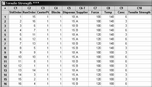
| Step 5. | Collect the data from the process as per the runs in the Design Matrix in Step 4. The runs should be conducted in random order to ensure that external Noise Variables don't affect the results. The corresponding Y value(s) for each run should be entered directly into the Design Matrix in the software. Be sure to keep a backup copy of all data.
| | | Step 6. | Run the DOE analysis in the software, including the terms in the model as follows:
Resolution III or IVJust the Factors, no Interactions Resolution V or VIFactors and 2-Factor Interactions (no 3-Factors or higher) Resolution VII and higherFactors, 2-Factor, and 3-Factor interactions (no 4-Factors or higher)
For Resolution VI and above it might be well worth considering a smaller Fraction.
| | | Step 7. | Most software packages give a visual representation of the effects of each of the Factors and Interactions, which can be invaluable in reducing the model (eliminating terms in the model with negligibly small coefficients). For the preceding 5-Factor example, the Pareto Chart of the effects is shown in Figure 7.18.3. The Design is a Resolution V Design, so terms for the 3-Factor Interactions and higher have been eliminated (pooled into the Error term).
Figure 7.18.3. An example of a Pareto Chart of Effects for the 5-Factor Fractional Factorial (output from Minitab v14). 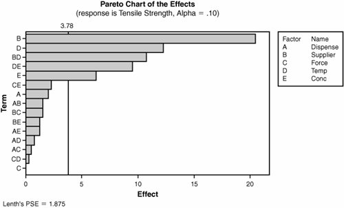
The focus should be on the highest order interaction(s) first. The vertical line at 3.78 in the figure represents the p-value cutoff point, in this case of 0.10. The higher value of 0.1 versus 0.05 is used to avoid eliminating any important terms accidentally. Usually it is best to eliminate a few of the bottom terms first and rerun the model advancing cautiously, a few terms dropped at a time, each time focusing on the terms to the left of the cutoff line. If this is done, the terms to remove from the model are all the terms including and below CE in the Figure.
In some analyses, the software does not allow the term for a Factor, such as C, to be removed from the model because the Factor in question appears in a higher order Interaction, such as AxC, that is not eliminated from the model. This is known as hierarchy. In this case, keep the Factor in place and it could be eliminated later or it might have to stay in the final model even if it does not contribute much by itself, only in the Interaction form.
For designs using Center Points, inspect the F-test for Curvature. If the p-value here is large, then there is no curvature effect to analyze and these can be pooled in to calculate the error term.
| | | Step 8. | Based on the preceding results, rerun the reduced model with only the significant effects. For the 5-Factor example, the results are shown in Figure 7.18.4. The analytical results are shown in Figure 7.18.5.
Figure 7.18.4. An example of a Pareto Chart of Effects for the reduced 5-Factor Fractional Factorial (output from Minitab v14). 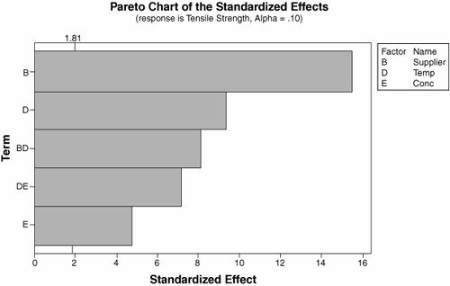
Figure 7.18.5. Numerical analysis for the reduced model of 5-Factor Fractional Factorial (output from Minitab v14).Factorial Fit: Tensile Strength versus Supplier, Temp, Conc | Estimated Effects and Coefficients for Tensile Strength (coded units) | Term | Effect | Coef | SE Coef | T | P | | Constant | | 65.250 | 0.6626 | 98.47 | 0.000 | | Supplier | 20.500 | 10.250 | 0.6626 | 15.47 | 0.000 | | Temp | 12.250 | 6.125 | 0.6626 | 9.24 | 0.000 | | Conc | 6.250 | 3.125 | 0.6626 | 4.72 | 0.001 | | Supplier*Temp | 10.750 | 5.375 | 0.6626 | 8.11 | 0.000 | | Temp*Conc | 9.500 | 4.750 | 0.6626 | 7.17 | 0.000 | | S = 2.65047 | R Sq = 97.89% | R Sq (adj) = 96.84% | | Analysis of Variance for Tensile Strength (coded units) | Source | DF | Seq SS | Adj SS | Adj MS | F | P | Main Effects | 3 | 2437.50 | 2437.50 | 812.500 | 115.66 | 0.000 | 2-Way Interactions | 2 | 823.25 | 823.25 | 411.625 | 58.59 | 0.000 | Residual Error | 10 | 70.25 | 70.25 | 7.025 | | | Lack of Fit | 2 | 7.25 | 7.25 | 3.625 | 0.46 | 0.647 | Pure Error | 8 | 63.00 | 63.00 | 7.875 | | | Total | 15 | 3331.00 | | | | |
At this point, the estimate of error should be good because ten pieces of information have been pooled to create it (DF = 10 for the Residual Error). According to the Lean Sigma analysis rule for p-values less than 0.05, this is as far as the analysis can go because all the p-values are below 0.05; so the associated Factors or Interactions are significant. However, it seems unlikely that all five remaining terms contribute to the big process picture. To understand their contribution, the Epsilon2 value should be calculated.
| | | Step 9. | Calculate Epsilon2 for each significant effect in the reduced model. In Minitab this is done using a separate function called the Balanced ANOVAmost other statistical software packages provide this. The results of this can be seen in Figure 7.18.6.
Figure 7.18.6. Epsilon2 Calculation for 5-Factor example (output from Minitab v14 with Epsilon2 hand calculated and typed in).Analysis of Variance for Tensile Strength |
|---|
Source | DF | SS | Eps-Sq |
|---|
Supplier | 1 | 1681.00 | 50.47 | Temp | 1 | 600.25 | 18.02 | Conc | 1 | 156.25 | 4.69 | Supplier*Temp | 1 | 462.25 | 13.88 | Temp*Conc | 1 | 361.00 | 10.84 | Error | 10 | 70.25 | 2.11 | Total | 15 | 3331.00 | |
It is clear from Figure 7.18.6 that all the remaining terms give meaningful contribution and should be kept in place for subsequent studies. If there were small contribution terms, a further reduction in the model would be conducted.
The final ANOVA table is the one already calculated and shown in Figure 7.18.5. The model explains 97.89% of the variation in the run data (R-Sq). The R-Sq(adj) value is close to the R-Sq value, which indicates that there aren't any redundant terms in the model. The Lack of Fit of the model is insignificant (the p-value is well above 0.05).
By closely controlling the three Factors in question (the Interactions are also taken care of if the Factors are controlled because they are comprised of the Factors), some 97.89% of the variability in the process is contained.
| Step 10. | Formulate conclusions and recommendations. The output of a Screening Design is not the optimum settings for all of the Factors identified; it merely identifies the process Factors that should be carried over to Characterization. Here the model is reduced significantly to the point that with so many terms pooled into the error, it might be possible to skip a Characterizing Design and go straight to an Optimizing Design.
Recommendations here would certainly include better control on the three identified Factors, but quite possibly a subsequent Optimizing DOE to determine the optimum settings for the three factors.
|
Other Options Some potential elements that were not considered here include Attribute Y data In the preceding analyses, all of the Ys were Continuous data, which made the statistics work more readily. If the Y is Attribute data, then quite often a key assumption of equal variance across the design is violated. To remove this issue, Attribute data has to be transformed, which is considered well beyond the scope of this book. Blocking on a Noise Variable The preceding examples did not include any Blocked Variables. Blocks are added if the Team is not sure that a potential Noise Variable could have an effect. The Noise Variable is tracked for the experiment and effectively entered as an additional X in the software. After the initial analysis run, when the first reductions are made the effect of Block would appear with its own p-value. If the p-value is above 0.1 then eliminate the Block from the model, because it has no effect. If the Block is important then it should be included in the model and subsequent analysis and experimental designs. Center Points and Curvature Center Points are useful to find good estimates of Error, but they also allow investigation of Curvature in the model. When the initial analysis is run, the Curvature should have its own p-value. Again if the p-value is high, then there is no significant effect from Curvature and the Curvature term can be eliminated from the reduced model going forward. Curvature is examined in greater detail in "DOEOptimizing" in this chapter.
|