4.2 Multiuser Detection via Robust Regression

4.2.1 System Model

For the sake of simplicity, we start the discussion in this chapter by focusing on a real-valued discrete-time synchronous CDMA signal model. At any time instant (until needed in Section 4.5, we will suppress the symbol index i ), the received signal is the superposition of K users' signals, plus the ambient noise, given by (see Section 2.2.1)

Equation 4.1

Equation 4.2

where, as before, , c _j,k {+1, “1}, is the normalized signature waveform of the k th user ; N is the processing gain; b _k {+1, “1} and A _k are, respectively, the data bit and the amplitude of the k th user; ; is a vector of independent and identically distributed (i.i.d.) ambient noise samples. As noted above, we adopt the commonly used two- term Gaussian mixture model for the additive noise samples { n _j }. The marginal probability density function (pdf) of this noise model has the form

Equation 4.3

with n > 0, 0 < and k > 1. Here the N (0, n ² ) term represents the nominal background noise, and the N (0, k n ² ) term represents the impulsive component, with representing the probability that impulses occur. It is usually of interest to study the effects of variation in the shape of a distribution on the performance of the system, by varying the parameters and k with fixed total noise variance

Equation 4.4

This model serves as an approximation to the more fundamental Middleton class A noise model [321, 600] and has been used extensively to model physical noise arising in radar, acoustic, and radio channels. In what follows we discuss some robust techniques for multiuser detection in non-Gaussian ambient noise CDMA channels, which are essentially robustified versions of the linear decorrelating multiuser detector.

4.2.2 Least-Squares Regression and Linear Decorrelator

Consider the synchronous signal model (4.2). Denote q _K A _k b _k . Then (4.2) can be rewritten as

Equation 4.5

or in matrix notation,

Equation 4.6

where . Consider the linear regression problem of estimating the K unknown parameters q ₁ , q ₂ , . . . , q _K from the N observations r ₁ , r ₂ , . . . , r _N in (4.5). Classically, this problem can be solved by minimizing the sum of squared errors (or squared residuals) [i.e., through the least-squares (LS) method]:

Equation 4.7

If n _j ~ N (0, s ² ), the pdf of the received signal r under the true parameters q is given by

Equation 4.8

It is easily seen from (4.8) that the maximum- likelihood estimate of q under the i.i.d. Gaussian noise assumption is given by the LS solution in (4.7). Upon differentiating (4.7), is then the solution to the following linear system equations

Equation 4.9

or in matrix form,

Equation 4.10

Define the cross-correlation matrix of the signature waveforms of all users as R S ^T S . Assuming that the user signature waveforms are linearly independent (i.e., S has a full column rank K ), R is invertible, and the LS solution to (4.9) or (4.10) is given by

Equation 4.11

We observe from (4.11) that the LS estimate is exactly the output of the linear decorrelating multiuser detector for the K users (cf. Proposition 2.1). This is not surprising, since the linear decorrelating detector gives the maximum likelihood estimate of the product of the amplitude and the data bit q _k = A _k b _k in Gaussian noise [296]. Given the estimate , the estimated amplitude and the data bit are then determined by

Equation 4.12

Equation 4.13

4.2.3 Robust Multiuser Detection via M -Regression

It is well known that the LS estimate is very sensitive to the tail behavior of the noise density [499]. Its performance depends significantly on the Gaussian assumption and even a slight deviation of the noise density from the Gaussian distribution can, in principle, cause a substantial degradation of the LS estimate. Since the linear decorrelating multiuser detector is in the form of the LS solution to a linear regression problem, it can be concluded that its performance is also sensitive to the tail behavior of the noise distribution. As will be demonstrated later, the performance of the linear decorrelating detector degrades substantially if the ambient noise deviates even slightly from a Gaussian distribution. In this section we consider some robust versions of the decorrelating multiuser detector, first developed in [553], which are nonlinear in nature. Robustness of an estimator refers to its performance insensitivity to small deviations in actual statistical behavior from the assumed underlying statistical model.

The LS estimate corresponding to (4.7) and (4.9) can be robustified by using the class of M -estimators proposed by Huber [203]. Instead of minimizing a sum of squared residuals as in (4.7), Huber proposed to minimize a sum of a less rapidly increasing function, r , of the residuals:

Equation 4.14

Suppose that r has a derivative , then the solution to (4.14) satisfies the implicit equation

Equation 4.15

or in vector form,

Equation 4.16

where for any x and denotes an all-zero vector. An estimator defined by (4.14) or (4.15) is called an M-estimator , from "maximum-likelihood-type estimator" [203], since the choice of r ( x ) = “log f ( x ) gives the ordinary maximum-likelihood estimator. If r is convex, then (4.14) and (4.15) are equivalent; otherwise , (4.15) is still very useful in searching for the solution to (4.14). To achieve robustness, it is necessary that y be bounded and continuous. Usually, to achieve high efficiency when the noise is actually Gaussian, we require that y ( x ) x for x small. Consistency of the estimate requires that E { y ( n _j )} = 0. Hence for symmetric noise densities , y is usually odd-symmetric. We next consider some specific choices of the penalty function r and the corresponding derivative y .

Linear Decorrelating Detector

The linear decorrelating detector, which is simply the LS estimator, corresponds to choosing the penalty function and its derivative, respectively, as

Equation 4.17

Equation 4.18

where a is any positive constant. Notice that the linear decorrelating detector is scale invariant.

Maximum-Likelihood Decorrelating Detector

Assume that the i.i.d. noise samples have a pdf f . Then the likelihood function of the received signal r under the true parameters q is given by

Equation 4.19

Therefore, the maximum-likelihood decorrelating detector in non-Gaussian noise with pdf f (in the sense that it gives the maximum-likelihood estimate of the product of the amplitude and data bit q _K A _k b _k ) is given by the M -estimator with the penalty function and its derivative, respectively, chosen as

Equation 4.20

Equation 4.21

Minimax Decorrelating Detector

We next consider a robust decorrelating detector in a minimax sense based on Huber's minimax M -estimator [203]. Huber considered the robust location estimation problem. Suppose that we have one-dimensional i.i.d. observations X ₁ , . . . , X _n . The observations belong to some subset c of the real line . A parametric model consists of a family of probability distributions F _q on c , where the unknown parameter q belongs to some parameter space Q . When estimating location in the model c = , Q = , the parametric model is F _q ( x ) = F ( x “ q ), and the M -estimator is determined by a y -function of the type y ( x , q ) = y ( x “ q ); that is, the M -estimate of the location parameter q is given by the solution to the equation

Equation 4.22

assuming that the noise distribution function belongs to the set of -contaminated Gaussian models given by

Equation 4.23

where 0 < < 1 is fixed and n ² is the variance of the nominal Gaussian distribution. It can be shown that within mild regularity, the asymptotic variance of an M -estimator of the location parameter q defined by (4.22) at a distribution function F P is given by [203]

Equation 4.24

Huber's idea was to minimize the maximal asymptotic variance over P , that is, to find the M -estimator y that satisfies

Equation 4.25

This is achieved by finding the least favorable distribution F , that is, the distribution function that minimizes the Fisher information

Equation 4.26

over all F P . Then yields the maximum-likelihood estimator for this least favorable distribution. Huber showed that the Fisher information (4.26) is minimized over P the distribution with pdf

Equation 4.27

where k , , and n are connected through

Equation 4.28

with , and . The corresponding minimax M -estimator is then determined by the Huber penalty function and its derivative, given, respectively, by

Equation 4.29

Equation 4.30

The minimax robust decorrelating detector is obtained by substituting r _H and y _H into (4.14) and (4.15).

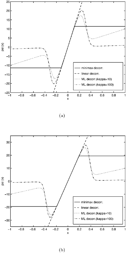
Assuming that the noise distribution has the -mixture density (4.3), in Fig. 4.1 we plot the y functions for the three types of decorrelating detectors discussed above for the cases = 0.1 and = 0.01, respectively. Note that for small measurement x , both y _ML ( x ) and y _H ( x ) are essentially linear, and they coincide with y _LS ( x ); for large measurement x , y _ML ( x ) approximates a blanker, whereas y _H ( x ) acts as a clipper. Thus the action of the nonlinear function y in the nonlinear decorrelators defined by (4.15) relative to the linear decorrelator defined by (4.9) is clear in this case. Namely, the linear decorrelator incorporates the residuals linearly into the signal estimate, whereas the nonlinear decorrelators incorporate small residuals linearly but blank or clip larger residuals that are likely to be the result of noise impulses.

Figure 4.1. The y functions for a linear decorrelator, maximum-likelihood decorrelator, and minimax decorrelator under the Gaussian mixture noise model. The variance of the nominal Gaussian distribution is n ² = 0.01. (a) = 0.1. The cutoff point for the Huber estimator is obtained by solving (4.28), resulting in g = 11.40. (b) = 0.01, g = 19.45