THE BAYESIAN APPROACH TO PROBABILITY

Chapter XI - Bayesian Data Mining and Knowledge Discovery
Data Mining: Opportunities and Challenges
by John Wang (ed)
Idea Group Publishing 2003

	Brought to you by Team-Fly

THE BAYESIAN APPROACH TO PROBABILITY

The classical approach of probability ties probability to the physical nature of the world. This means that if we toss a coin, the probability of getting heads or tails is intrinsically linked to the physical properties of the coin. Under this interpretation, we could estimate the "probability of getting heads" as the frequency of heads after repeating the experiment a certain number of times. The (weak) Law of Large Numbers states that when the number of random observations of a certain event is very large, the relative frequency of the observations is a near exact estimate of the probability of the event. Since frequencies can be measured, this frequentist interpretation of probability seemed to be an objective measure for dealing with random phenomena.

There are many situations in which the frequency definition of probability exhibits its limited validity. Although the classical (frequentist) approach seems to be a good way of estimating probabilities, difficulties surface when facing situations in which experiments are not possible. For example, when trying to answer the question of "Who is going to be the next President of the United States of America?", the frequentist approach fails to provide an answer; the event has an associated probability, but there is no possible way of experimenting and measuring the relative frequencies because the event has a single occurrence. And there are many other cases in which a frequency approach is not applicable or is, at least, far-fetched. Why should we have to think of probability in terms of many repetitions of an experiment that never happened? As Sivia (1996) mentions, we are at liberty to think about a problem in any way that facilitates a solution or our understanding of it, but having to seek a frequentist interpretation for every data analysis problem seems rather perverse.

The Bayesian approach, instead, provides an elegant framework to deal with this kind of probability problems. To Bayesians, the probability of a certain event represents the degree of belief that such event will happen. We don't need to think of probabilities as frequency distributions probability measures the degree of personal belief. Such belief is therefore governed by a probability distribution that can be updated by making use of the observed data. To do so, however, Bayesians address data analysis from a different perspective; i.e., the personal belief in the occurrence of a certain event starts with a given distribution, which stands before any data is considered and is therefore known as prior distribution. Observational data is incorporated into the data analysis process in order to obtain a posterior probability distribution by updating our prior belief. But how do we perform this update of our prior belief? And besides, where does the name Bayesian come from?

Bayesian thinking has its roots in the question of how to reason in situations in which it is not possible to argue with certainty, and in the difference between inductive and deductive logic. The problem of inductive reasoning has puzzled philosophers since the time of Aristotle, as a way of inferring universal laws from a finite number of cases, as opposed to deductive logic, the kind of reasoning typically used in mathematics. Deductive logic is based on deriving the conclusion from the implicit content of its premises, so that if the premises are true, then the conclusion is necessarily true. We can therefore derive results by applying a set of well-defined rules. Games of chance fall into this category as well. If we know that an unbiased die is rolled five times, we can calculate the chances of getting three ones, for example.

Inductive reasoning tackles a different problem, actually the reverse of the above situation; i.e., given that a finite number of effects can be observed, derive from them a general (causal) law capable of explaining each and all of the effects (premises) from which it was drawn. Going back to the previous example, inductive reasoning would try to explain whether the rolled die is biased or not after observing the outcome of five repeated throws.

Bayes' Theorem

Bayes' Theorem is derived from a simple reordering of terms in the product rule of probability:

If we replace B by H (a hypothesis under consideration) and A by D (the evidence, or set of observational data), we get:

Note that:

• P(H∣D) is the probability of a certain hypothesis based on a set of observational data given a certain context (posterior probability of hypothesis H);

• P(D∣H) is the likelihood of the observations given a certain hypothesis in a given context;

• P(H) is the intrinsic probability of hypothesis H, before considering the evidence D (prior probability);

• P(D) is the probability of the observations, independent of the hypothesis, that can be interpreted as a normalizing constant rendering P(H/D) to a value interval of [0,1].

Bayes' Theorem can then be reformulated in the following way: the probability of a certain hypothesis given a set of observations in a given context depends on its prior probability and on the likelihood that the observations will fit the hypothesis.

This means that the probability of the hypothesis is being updated by the likelihood of the observed data. The result of the Bayesian data analysis process is the posterior probability distribution of the hypothesis that represents a revision of the prior distribution in the light of the evidence provided by the data.

Conjugate Prior Distributions

Let us first reformulate Bayes' Theorem in terms of probability distributions. As such, Bayes' formula can be rewritten as:

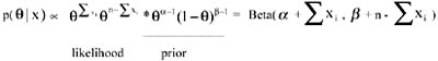
where the prior p(θ) on the unknown parameter θ characterizes knowledge or beliefs about θ before seeing the data; the likelihood function p(x∣θ) summarizes the sample information about θ.

In order to assess the prior distribution of θ, many Bayesian problems make use of the notion of conjugacy. For each of the most popular statistical families, there exists a family of distributions for the parameter such that, if the prior distribution is chosen to be a member of the family, then the posterior distribution will also be a member of that family. Such a family of distributions is called a conjugate family. Choosing a prior distribution from that family will typically simplify the computation of the posterior.

For example, suppose that X1, X2,..Xn form a random sample drawn from a Bernoulli distribution for which the parameter θ is unknown. Suppose that we choose a Beta distribution for prior, with parameters α and β, both > 0 Then the posterior distribution of θ given the sample observations is also a Beta, with parameters

As can be seen in the previous expression, given that the likelihood is a binomial distribution, by choosing the prior as a Beta distribution, the posterior distribution can be obtained without the need of integrating a rather complex function. Although this is a very convenient approach, in many practical problems there is no way of approximating our prior beliefs by means of a "nice" (conjugate) prior distribution.

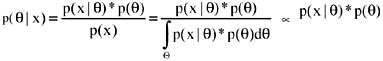
Critique of the Bayesian Framework

The Bayesian approach did not come without difficulties. The concerns regarding subjectivity of its treatment of probability is understandable. Under the belief interpretation, probability is not an objective property of some physical setting but is conditional to the prior assumptions and experience of the learning system. The prior probability distribution can arise from previously collected observations, but if the data is not available, it should be derived from the subjective assessment of some domain expert. According to this personal, or subjective, interpretation of probability, the probability that a person assigns to a possible outcome of some process represents his/her judgment of the likelihood that the outcome will be obtained. This subjective interpretation can be formalized, based on certain conditions of consistency. However, as DeGroot (1986) describes, the requirement that a person's judgment of the relative likelihood of a large number of events be completely consistent and free of inconsistencies is humanly unattainable. And besides, a subjective interpretation may not provide a common basis for an objective theory about a certain topic of interest. Two different persons may have two different interpretations and may not reach a common evaluation of the state of knowledge. Now, how much does this subjectivity issue affect the Bayesian framework? As Sivia (1996) points out, the Bayesian view is that a probability does indeed represent how much do we believe that a certain event is true, but this belief should be based on all the relevant information available. This is not the same as subjectivity; it simply means that probabilities are conditional on the prior assumptions and that these assumptions must be stated explicitly. Janes (1996) explains that objectivity only demands that two individuals who are given the same information and who reason according to the rules of probability theory should make the same probability assignment. Interestingly enough, Cox (1946) studied the quantitative rules necessary for logical and consistent reasoning and showed that plausible reasoning and calculus of beliefs map exactly into the axioms of probability theory. He found that the only rules that met the requirements for logical and consistent reasoning were those derived from probability theory.

The other source of criticism is based on scalability. Within the field of artificial intelligence, for example, the use of Bayesian methods in expert systems was criticized because the approach did not scale well for real-world problems. To visualize these scalability issues, let us consider the typical problems faced when trying to apply the Bayesian framework. The Bayes' formula can be expressed as:

Note that the normalizing factor p(x) is calculated by integrating over all the possible values of θ. But what happens when we deal with multidimensional parameters, that is that ? In such case, the normalizing factor must be calculated as , and the resulting expressions may not have a straightforward analytical solution and, in the worst case, may be computationally infeasible. Similar situations arise when trying to calculate marginal densities or expected values. In the case of expectation, the goal of the analysis may be to obtain the expected value of a function g(θ) for which we have:

As can be observed, we encounter a similar kind of problem as before. For high-dimensional spaces, it is usually impossible to evaluate these expressions analytically, and traditional numerical integration methods are far too computationally expensive to be of any practical use.

Luckily, new developments in simulation during the last decade have mitigated much of the previous criticism. The inherent scalability problems of traditional Bayesian analysis, due to the complexity of integrating expressions over high-dimensional distributions, have met an elegant solution framework. The introduction of Markov Chain Monte Carlo methods (MCMC) in the last few years has provided enormous scope for realistic Bayesian modeling (more on this later in this chapter).

	Brought to you by Team-Fly