RESULTS

Chapter II - Control of Inductive Bias in Supervised Learning Using Evolutionary Computation A Wrapper-Based Approach
Data Mining: Opportunities and Challenges
by John Wang (ed)
Idea Group Publishing 2003

	Brought to you by Team-Fly

Synthetic and Small-Scale Data Mining Problems

This section presents experimental results with comparisons to existing inductive learning systems (Kohavi, Sommerfield & Dougherty, 1996): decision trees, traditional regression-based methods as adapted to time series prediction, and non-modular probabilistic networks (both a temporal and ARIMA-type ANNs).

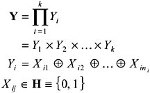
The Modular Parity Problem

Figure 3 shows the classification accuracy in percent for specialist and moderator output for the concept:

Figure 3: Mean classification accuracy of specialists vs. moderators for all (52) partitions of 5-attribute modular parity problem.

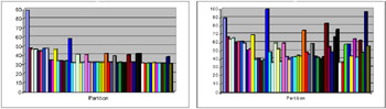
All mixture models are trained using 24 hidden units, distributed across all specialists and moderators. When used as a heuristic evaluation function for partition search, the HME metric documented in the previous section finds the best partition for the 5-attribute problem (shown below) as well as 6, 7, and 8, with no backtracking, and indicates that an MS-HME model should be used.

This section documents improvements in classification accuracy as achieved by attribute partitioning. Figure 3 shows how the optimum partition {{1,2,3}{4,5}} for the concept:

achieves the best specialist performance for any size-2 partition.

Figure 3 shows how this allows it to achieve the best moderator performance overall. Empirically, "good splits" especially descendants and ancestors of the optimal one, i.e., members of its schema (Goldberg, 1989) tend to perform well.

As documented in the background section, partition search is able to find Partition #16, {{1,2,3}{4,5}} (the optimum partition) after expanding all of the 2-subset partitions. This reduces B_n evaluations to Θ(2ⁿ); attribute partitioning therefore remains an intractable problem, but is more feasible for small to moderate numbers of attributes (30-40 can be handled by high-performance computers, instead of 15-20 using exhaustive search). Approximation algorithms for polynomial-time evaluation (Cormen et al., 2001) are currently being investigated by the author.

For experiments using specialist-moderator networks on a musical tune classification problem synthetic data quantized from real-world audio recordings the interested reader is referred to Hsu et al. (2000).

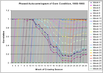
Application: Crop Condition Monitoring

Figure 4 visualizes a heterogeneous time series. The lines shown are phased autocorrelograms, or plots of autocorrelation shifted in time, for (subjective) weekly crop condition estimates, averaged from 1985-1995 for the state of Illinois. Each point represents the correlation between one week's mean estimate and the mean estimate for a subsequent week. Each line contains the correlation between values for a particular week and all subsequent weeks. The data is heterogeneous because it contains both an autoregressive pattern (the linear increments in autocorrelation for the first ten weeks) and a moving average pattern (the larger, unevenly spaced increments from 0.4 to about 0.95 in the rightmost column). The autoregressive process, which can be represented by a time-delay model, expresses weather "memory" (correlating early and late drought); the moving average process, which can be represented by an exponential trace model, physiological damage from drought. Task decomposition can improve performance here by isolating the AR and MA components for identification and application of the correct specialized architecture a time delay neural network (Haykin, 1999; Lang et al., 1990) or simple recurrent network (Princip & Lefebvre, 2001), respectively.

Figure 4: Phased autocorrelogram (plot of autocorrelation shifted over time) for crop condition (average quantized estimates).

We applied a simple mixture model to reduce variance in ANN-based classifiers. A paired t-test with 10 degrees of freedom (for 11-year cross-validation over the weekly predictions) indicates significance at the level of p < 0.004 for the moderator versus TDNN and at the level of p < 0.0002 for the moderator versus IR. The null hypothesis is rejected at the 95% level of confidence for TDNN outperforming IR (p < 0.09), which is consistent with the hypothesis that an MS-HME network yields a performance boost over either network type alone. This result, however, is based on relatively few samples (in terms of weeks per year) and very coarse spatial granularity (statewide averages).

Table 3 summarizes the performance of an MS-HME network versus that of other induction algorithms from MLC++ (Kohavi et al., 1996) on the crop condition monitoring problem. This experiment illustrates the usefulness of learning task decomposition over heterogeneous time series. The improved learning results due to application of multiple models (TDNN and IR specialists) and a mixture model (the Gamma network moderator). Reports from the literature on common statistical models for time series (Box et al., 1994; Gershenfeld & Weigend, 1994; Neal, 1996) and experience with the (highly heterogeneous) test bed domains documented here bears out the idea that "fitting the right tool to each job" is critical.

Table 3: Performance of a HME-type mixture model compared with that of other inducers on the crop condition monitoring problem

	Classification Accuracy, Crop Condition Monitoring (%)
	Training				Cross Validation
Inducer	Min	Mean	Max	StdDev	Min	Mean	Max	StdDev
ID3	100.0	100.0	100.0	0.00	33.3	55.6	82.4	17.51
ID3, bagged	99.7	99.9	100.0	0.15	30.3	58.2	88.2	18.30
ID3, boosted	100.0	100.0	100.0	0.00	33.3	55.6	82.4	17.51
C5.0	90.7	91.7	93.2	0.75	38.7	58.7	81.8	14.30
C5.0, boosted	98.8	99.7	100.0	0.40	38.7	60.9	79.4	13.06
IBL	93.4	94.7	96.7	0.80	33.3	59.2	73.5	11.91
Discrete Na ve-Bayes	74.0	77.4	81.8	2.16	38.7	68.4	96.7	22.85
DNB, bagged	73.4	76.8	80.9	2.35	38.7	70.8	93.9	19.63
DNB, boosted	76.7	78.7	81.5	1.83	38.7	69.7	96.7	21.92
PEBLS	91.6	94.2	96.4	1.68	27.3	58.1	76.5	14.24
IR Expert	91.0	93.7	97.2	1.67	41.9	72.8	94.1	20.45
TDNN Expert	91.9	96.8	99.7	2.02	48.4	74.8	93.8	14.40
Pseudo-HME	98.2	98.9	100.0	0.54	52.9	79.0	96.9	14.99

Application: Loss Ratio Prediction in Automobile Insurance Pricing

Table 4 summarizes the performance of the ID3 decision tree induction algorithm and the state-space search-based feature subset selection (FSS) wrapper in MLC++ (Kohavi et al., 1996) compared to that of a genetic wrapper for feature selection. This system is documented in detail in Hsu, Welge, Redman, and Clutter (2002). We used a version of ALLVAR-2, a data set for decision support in automobile insurance policy pricing. This data set was used for clustering and classification and initially contained 471-attribute record for each of over 300,000 automobile insurance policies, with five bins of loss ratio as a prediction target. Wall clock time for the Jenesis and FSS-ID3 wrappers was comparable. As the table shows, both the Jenesis wrapper and the MLC++ wrapper (using ID3 as the wrapped inducer) produce significant improvements over unwrapped ID3 in classification accuracy and very large reductions in the number of attributes used. The test set accuracy and the number of selected attributes are averaged over five cross validation folds (70 aggregate test cases each). Results for data sets from the Irvine database repository that are known to contain irrelevant attributes are also positive. Table 10 presents more descriptive statistics on the five-way cross-validated performance of ID3, FSS-ID3 (the MLC++ implementation of ID3 with its feature subset selection wrapper), and Jenesis. Severe overfitting is quite evident for ID3, based on the difference between training and test set error (perfect purity is achieved in all five folds) and the larger number of attributes actually used compared to the wrappers. Jenesis and FSS-ID3 perform comparably in terms of test set error, though FSS-ID3 has less difference between training and test set error. and Jenesis is less likely to overprune the attribute subset. Note that FSS-ID3 consistently selects the fewest attributes, but still overfits (Jenesis achieves lower test set error in three of five cross validation cases). The test set errors of Jenesis and FSS-ID3 are not significantly different, so generalization quality is not conclusively distinguishable in this case. We note, however, that excessively shrinking the subset indicates a significant tradeoff regarding generalization quality. The classification model was used to audit an existing rule-based classification system over the same instance space, and to calibrate an underwriting model (to guide pricing decisions for policies) for an experimental market.

Table 4: Results from Jenesis for One Company (5-way cross validation), representative data sets

		Cross Validation Segment
		0	1	2	3	4	Mean	Stdev
Training Set Accuracy (%)	ID3	100.0	100.0	100.0	100.0	100.0	100.0	0.00
	FSS-ID3	55.00	54.29	67.86	50.36	60.71	57.64	6.08
	Jenesis	65.71	67.14	71.43	71.43	55.71	66.29	5.76
Test Set Accuracy (%)	ID3	41.43	42.86	28.57	41.43	44.29	39.71	5.67
	FSS-ID3	48.57	35.71	34.29	47.14	54.29	44.00	7.74
	Jenesis	41.43	42.86	31.43	52.86	55.71	44.86	8.69
Attributes Selected	ID3	35	35	37	40	35	36.40	1.96
	FSS-ID3	7	8	7	13	18	10.60	4.32
	Jenesis	20	19	22	20	23	20.80	1.47

We have observed that the aggregation method scales well across lines of business (the indemnity and non-indemnity companies) and states. This was demonstrated using many of our decision tree experiments and visualizations using ALLVAR-2 samples and subsamples by state.

	Brought to you by Team-Fly