15.

[Cover] [Contents] [Index]

Page 110

1 to 4 can be coded as 00, 01, 10, and 11, respectively. The spread approach, however, has the advantage that the result of classification is directly mapped on to the output vector, and so this approach is more widely used. For example, in the previous four-class case, if an input pattern belongs to class 3, the output vector will be coded as (0, 0, 1, 0). Such a data representation can enlarge the Hamming distance between individual vectors. For any two words x and y the Hamming distance d(x, y) is defined by:

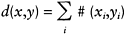(3.10)

where x_i and y_i denote alphabets at location i and 1≤i≤n, and the function #(a, b)=1 if a≠b, and 0 otherwise.

3.1.3 Decision boundaries in feature space

A classic example showing the relationship between the multilayer perceptron network structure and the location and shape of decision boundaries in feature space, is the problem of classifying the output from a simple XOR operator. Figure 3.3a shows the results of the XOR operation and the corresponding positions of the required decision boundaries are shown in Figure 3.3b.

It can be shown that a 2|0|2 network (i.e. two input neurones, no hidden neurones, and two output neurones in case of spread coding) cannot solve this classification problem because this network is only able to construct a single straight-line decision boundary. The XOR classification problem can only be solved if the network contains a hidden layer of neurones. Moreover, different sizes of neural networks (i.e. with different numbers of hidden neurones) will, in general, produce different decision boundaries. A larger network has the potential to form more complicated decision boundaries than a smaller network. To demonstrate this point, we use a three-class classification problem (modified from the XOR problem) over a two-dimensional domain within the data range of [0, 1]. Each dimension is further partitioned into 100×100 subsquares. Only five training patterns are used, and the corresponding locations are illustrated in Figure 3.3c.

Two networks are used for this experiment. One has a 2|3|3 structure, with fifteen weights (2×3=6 weights connecting the input and hidden layers, and 3×3=9 weights connecting the hidden and output layers) and the other has a 2|40|60|3 structure, with 2660 weights. The output vector is coded using the spread approach. There are two neurones in the input layer because the feature space shown in Figure 3.3c is two-dimensional. There are three neurones in the output layers because there are three classes in the problem shown in Figure 3.3c. The results shown

[Cover] [Contents] [Index]