The Formula Node

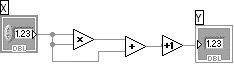
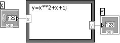
Now that you know about LabVIEW's four main control flow structures, we'll introduce a structure that doesn't affect program flow. The Formula Node is a resizable box that you use to enter algebraic formulas directly into the block diagram. You will find this feature extremely useful when you have a long formula to solve. For example, consider the fairly simple equation, y = x² + x + 1. Even for this simple formula, if you implement this equation using regular LabVIEW arithmetic functions, the block diagram is a little bit harder to follow than the text equations (see Figure 6.67).

Figure 6.67. A snippet of code that we can convert to a formula and put inside a Formula Node, as shown in Figure 6.68

You can implement the same equation using a Formula Node, as shown in Figure 6.68.^[1]

^[1] In versions prior to LabVIEW 6.0, the exponentiation operator for the Formula Node was the ^ symbol. In LabVIEW 6.0 and greater, the ^ symbol means something else entirely (bit-wise XOR), and the ** symbol is exponentiation.

Figure 6.68. A Formula Node containing a formula derived from the code snippet in Figure 6.67

With the Formula Node, you can directly enter a formula or formulas, in lieu of creating complex block diagram subsections. Simply enter the formula inside the box. You create the input and output terminals of the Formula Node by popping up on the border of the node and choosing Add Input or Add Output from the pop-up menu. Then enter variable names into the input and output terminals. Names are case sensitive, and each formula statement must terminate with a semicolon (;).

You will find the Formula Node in the Programming>>Structures subpalette of the Functions palette.

These operators and functions are available inside the Formula Node.

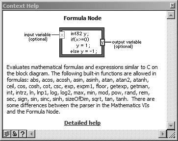
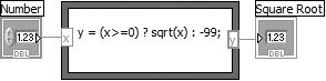
To get detailed information on the Formula Node syntax, open the Help window and place the cursor over the formula node. The Help window will look like Figure 6.69. Click on the Detailed help link to open the LabVIEW help file and then follow the Formula Node Syntax link.

Figure 6.69. The Context Help window showing detailed information about the Formula Node

The following example shows a conditional branching that you could perform inside a Formula Node. Consider the following code fragment, similar to Activity 6-3, which computes the square root of x if x is positive, and assigns the result to y. If x is negative, the code assigns value of 99 to y.

if (x >= 0) then       y = sqrt(x) else       y = -99 end if 

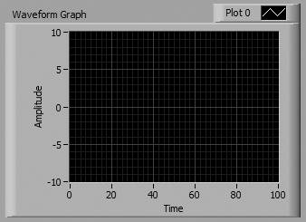
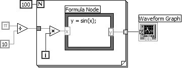
You can implement the code fragment using a Formula Node, as shown in Figure 6.70.

Figure 6.70. A Formula Node formula with some of its syntax elements annotated

Activity 6-5: Formula Fun

You will build a VI that uses the Formula Node to evaluate the equation y = sin(x), and graph the results.

1.	Open a new panel. Select Waveform Graph from the Modern>>Graph subpalette of the Controls palette (see Figure 6.71). Label it Graph. You'll learn all about graphs in Chapter 8, but this activity would be kind of dull without a nice pictorial representation, so we thought we'd give you a taste of them. Figure 6.71. The front panel of the VI you will build during this activity
2.	Build the block diagram shown in Figure 6.72. Figure 6.72. The block diagram of the VI you will build during this activity With the Formula Node (Structures palette), you can directly enter mathematical formulas. Create the input terminal by popping up on the border and choosing Add Input from the pop-up menu; then create the output terminal by choosing Add Output from the pop-up menu. When you create an input or output terminal, you must give it a variable name. The variable name must exactly match the one you use in the formula. Remember, variable names are case sensitive. Notice that a semicolon (;) must terminate each statement in the formula node. Pi Constant The π constant is located in the Functions>>Programming>>Numeric>>Math and Scientific Constants palette. During each iteration, the VI multiplies the iteration terminal value by π/10. The multiplication result is wired to the Formula Node, which computes the sine of the result. The VI then stores the result in an array at the For Loop border. (You will learn all about arrays in Chapter 7. Then you will see why you can wire array data out of a For Loop, while scalar data comes out of a While Loop by default.) After the For Loop finishes executing, the VI plots the array.
3.	Return to the front panel and run the VI. Note that you could also use the existing Sine function (Functions>>Numeric>>Trigonometric palette) to do the same thing as the Formula Node in this activity, but LabVIEW does not have built-in functions for every formula you'll need, and we wanted to give you the practice.
4.	Save the VI in your MYWORK directory and name it Formula Node Exercise.vi. Close the VI.

VI Logic

timebase = PI/10 for i = 0 to 99       x = i * timebase       y = sin(x)       array[i] = y next i Graph (array)