Advanced Data Acquisition
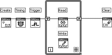
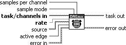
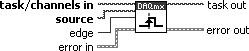
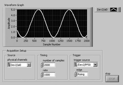
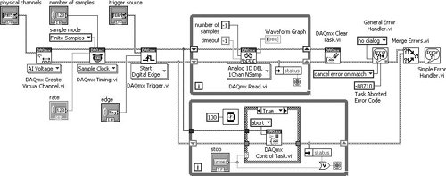
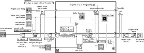
| In this section, we'll look at some more advanced scenarios in data acquisition, such as timing and triggering, continuous data acquisition, streaming data to disk, and counting events. DAQmx Timing and DAQmx TriggerAs we mentioned at the beginning of this section, you can configure timing and triggering options before you start using your task. In this case, your NI-DAQmx applications will be logically organized something like Figure 11.54. Figure 11.54. Block diagram showing the logical organization of a typical NI-DAQmx application Both DAQmx Timing and DAQmx Trigger are polymorphic VIs. After placing them on the block diagram, use the Polymorphic VI Selector ring to choose a specific instance. Figure 11.55. DAQmx Timing Figure 11.56. DAQmx Trigger DAQmx Timing (Measurement I/O>> DAQmx Data Acquisition palette) configures the number of samples to acquire or generate and creates a buffer when needed. The instances of this polymorphic VI correspond to the type of timing to use for the task. The DAQmx Timing properties include all timing options included in this VI and additional timing options. DAQmx Trigger (Measurement I/O>>DAQmx Data Acquisition palette) configures triggering for the task. The instances of this polymorphic VI correspond to the trigger and trigger type to configure. The DAQmx Trigger properties include all triggering options included in this VI and additional triggering options. Now, let's take what you've learned about NI-DAQmx timing and triggering and build a VI using both of these features. Activity 11-6: Triggered Data Acquisition Using TasksYou will now learn how to use the DAQmx Timing and DAQmx Triggering VIs to acquire a buffered analog input signal when triggered by a digital line. Each time the trigger event occurs, you will read the acquired data and display it in a waveform graph. You will use the VI created in Activity 11-4 to generate the trigger signal needed for acquiring the data and the VI created in Activity 11-5 to generate the analog signal that will be acquired.
For this activity to run, you will need a physical NI-DAQmx device. The signal connection (wiring) table is at the end of this activity.
Congratulations. You've just created some very powerful data acquisition tools! You will be able to use these VIs, and variations of them, to achieve all sorts of functionalityyour imagination is the limit! Multichannel AcquisitionEarlier, you did an activity where you acquired several channels at once. This is known as multi-channel acquisition. This is a good time to point out the distinction between scan rate and sampling rate:
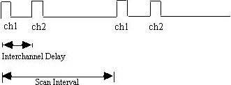
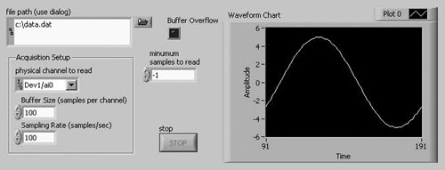
On DAQ boards, we usually talk about setting the scan rate. Most of the time scan rate = sampling rate. However, that is not always true, and there is an important limitation of multi-channel I/O that you need to be aware of. If you set a high scan rate for multiple channels, and observe the data from each channel over actual time (not over array index values), you will notice a successive phase delay between each channel. Why is this? Most DAQ devices can only perform one A/D conversion at a time. That's why it's called scanning: The data at the input channels is digitized sequentially one channel at a time. A delay, called the interchannel delay (depicted in Figure 11.59), arises between each channel sample. Figure 11.59. Interchannel delay By default, the interchannel delay is as small as possible, but is highly dependent on the DAQ device. A few DAQ devices, such as the National Instruments S Series devices, do support simultaneous sampling of channels. Other devices support either interval scanning or round robin scanning (depicted in Figure 11.60). Devices that support interval scanning have a much smaller interchannel delay than those that use round robin scanning. Figure 11.60. Interval scanning (left) and round robin scanning (right)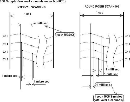 With DC and low-frequency signals, this phase delay in scans is generally not a problem. The interchannel delay may be so much smaller than the scan period that the DAQ device appears to virtually sample each channel simultaneously: for example, the interchannel delay may be in the microsecond range and the sampling rate may be 1 scan/sec. However, at higher frequencies, the delay can be very noticeable and may present measurement problems if you are depending on the signals being synchronized. Continuous Data AcquisitionContinuous data acquisition, or real-time data acquisition, returns data from an acquisition in progress without interrupting the acquisition. This approach usually involves a circular buffer scheme, as shown in Figure 11.61. You specify the size of a large circular buffer. The DAQ device collects data and stores the data in this buffer. When the buffer is full, the DAQ device starts writing data at the beginning of the buffer (writing over the previously stored data, whether or not it has been read by LabVIEW). This process continues until the system acquires the specified number of samples, LabVIEW clears the operation, or an error occurs. Continuous data acquisition is useful for applications such as streaming data to disk and displaying data in real time. Figure 11.61. Circular buffer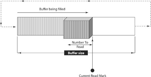 In the next activity, you will create a VI that acquires data continuously and plots the most recent data. Activity 11-7: Continuous AcquisitionYou will create a VI that performs a continuous acquisition by configuring NI-DAQmx to acquire data into a circular buffer. You will read data out of the circular buffer as it becomes available and display it on a waveform chart. You will also validate that you are reading data fast enough (and that the buffer has not overflowed, causing data loss) by checking whether the amount of data available is less than the size of the circular buffer.
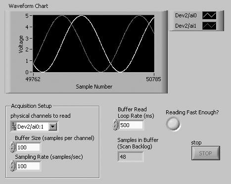
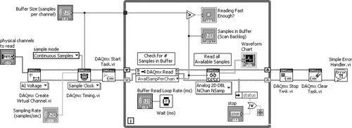
Now configure the acquisition setup parameters on the front panel and run your VI. Note that your loop rate must be fast enough that the buffer does not overflow! Adjust the Buffer Read Loop Rate so that each loop cycle time is less than the time it takes to fill the buffer. You can calculate the time that it takes to fill the buffer using the following, simple equation: Time to Fill the Buffer = Buffer Size / Sampling Rate The Continuous Acquisition VI that you just created is designed to run continuously, or "forever." In order to accomplish this without running out of memory, a fixed-length buffer is allocated, filled up with samples of data from beginning to end, and then the data at the beginning is overwritten as the buffer is filled up again. As an example, suppose this VI were run with a buffer size of 10 and the sampling rate was once per second. Here are snapshots of how the buffer is being filled up with data: Before the VI is run, the buffer is empty: After one second, one sample is filled: After nine seconds, the buffer is almost full: After twelve seconds, the buffer has filled up and the data at the beginning is being overwritten: Why the Samples in Buffer (Scan Backlog) indicator? It's pretty useful to know if LabVIEW is keeping up with reading the data. If the buffer fills up faster than your VI can retrieve the data in it, you will start losing some of this data, because the buffer will be overwritten. Are you ready for some TLAs (that's "Three-Letter Acronyms," as you learned in Chapter 10)? You'll definitely want to refer back to the "DAQ and Other Data Acquisition Acronyms" section of Chapter 10, if you want to understand these next two paragraphs! The Continuous Acquisition VI you just made takes advantage of NI-DAQmx's hardware timing and memory handling capabilities. If, while your continuous acquisition task is running, an OS event ties up the CPU, NI-DAQmx will use the DAQ device's buffer and DMA capability (if any) to continue collecting data without any CPU involvement. DMA allows the DAQ hardware to write directly to the computer's memory, even if the processor is tied up. If the OS event interrupts the CPU longer than the on-board FIFO buffer and the DMA buffer can handle, only then will NI-DAQmx lose data samples. This can best be understood by referring to the previous four snapshots of the buffer. First, assume the DAQ device has no on-board FIFO, but it has DMA capability. Ideally, the DAQ hardware will write data into the buffer continuously, and LabVIEW will be continuously reading a few samples behind the last sample written to the buffer. Suppose the CPU gets tied up after one second, and LabVIEW has read the first sample. When the CPU is tied up, the DAQ device can write to this buffer, but LabVIEW can't read from the buffer. If after twelve seconds, the CPU is still tied up, then LabVIEW has missed the data in the second slot from the left when it contained good data (light gray). Streaming Data to a FileYou have already written exercises that send data to a spreadsheet file. In those exercises, LabVIEW converted the data to a spreadsheet file format and stored it in an ASCII file after the acquisition completed. A different and sometimes more efficient approach is to write small pieces of the data to the hard disk while the acquisition is still in progress. This type of file I/O is called streaming. An advantage of streaming data to file is that it's fast, so you can execute continuous acquisition applications and yet have a stored copy of all the sampled data. Another reason to stream data to file is that if you are acquiring data continuously at a very fast rate for a long period of time, you will likely run out of memory. Unless your data rate is very low (for example, less than 10 samples/sec), you normally will need to stream to binary, not ASCII, files. Binary files are much smaller in size and allow you to write data more compactly than is possible with text files. With continuous applications, the speed at which LabVIEW can retrieve data from the acquisition buffer and then stream it to disk is crucial. You must be able to read and stream the data fast enough so that the DAQ device does not attempt to overwrite unread data in the circular buffer. To increase the efficiency of the data retrieval, you should avoid executing other functions, such as analysis functions, while the acquisition is in progress. Also, you can configure DAQmx Read to return raw binary data rather than voltage data (by selecting one of the raw data modes beneath More>>Raw>> from its Polymorphic VI Selector). This increases the efficiency of the retrieval as well as the streaming. When you configure DAQmx Read to produce only binary data, it can return the data faster to the buffer than if you used the analog waveform or voltage modes. One disadvantage to reading and streaming binary data is that users of other applications cannot easily read the file. You can easily modify a continuous DAQ VI to incorporate the streaming feature. Although you may not have used binary files before, you can still build the VI in the following example. We will be discussing binary and other file types in Chapter 14. Activity 11-8: Streaming Data to FileIn this activity, you will modify Continuous Acquisition.vi, which you created in Activity 11-7, so that it streams data to file.
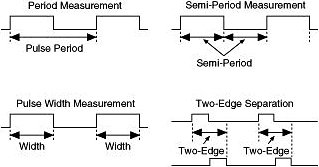
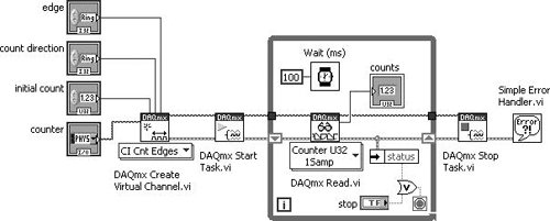
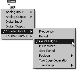
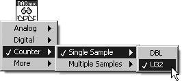
To see the data written to disk, use the companion example VI Read Streamed Data File.vi, shown in Figures 11.67 and 11.68, found on the CD at EVERYONE\CH11. We've provided this VI for you because it involves a few concepts, such as type casting data, which you have not yet learned about. (You will learn about the Type Cast function in Chapter 14.) Figure 11.67. Read Streamed Data File.vi front panel, used for reading the data files you create during this activity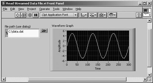 Figure 11.68. Read Streamed Data File.vi block diagram, used for reading the data files you create during this activity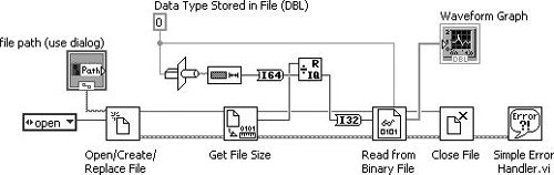 Run this VI, choosing the filename you used in the previous VI. Notice that the first VI, which streams data, doesn't attempt to graph the data. The point of streaming is to acquire data to the disk fastand look at it later. Take a look at the VI's block diagram to see how it reads the binary data from the file (see Figure 11.68). Some of the stuff should make sense, but some of it might puzzle you. Don't waste time trying to figure out the puzzling stuff yet. We'll get to it later. Counting Frequency and EventsAs you know, digital signals can be either off or on, 0 or 1, true or false. Despite the fact that digital signals are bi-polar, they actually have a lot of interesting personality! Digital signals can have a wealth of timing and event characteristics. For example, how many times has a digital line changed states, at what rate is it changing state, and for what amount of time has it been in the on state versus the off state? You can actually measure these digital signal characteristics and generate signals having the characteristics of your choosing! However, trying to measure and generate digital signal timing and events using only software is very limited and complicatedit just doesn't work very well because software loops run slowly and unsteadily when compared to most digital signals. Fortunately, there is a special type of signal conditioning hardware for acquiring and generating digital timing and event signals: It is called the counter (or counter/timer). A counter is an ASIC (Application Specific Integrated Circuit) computer chip that is designed for measuring and generating digital timing and events. It is likely that your multifunction DAQ device will have one or two counters on it. There also exist specific Counter/Timer Devices that have several counters (for example, 4, 8, or 16 counters) and several digital I/O lines but no analog I/O. Measuring Digital Events and Timing with CountersSo, what kinds of counter measurements might you want to make? Table 11.3 lists common counter measurements, some of which are also illustrated in Figure 11.69.
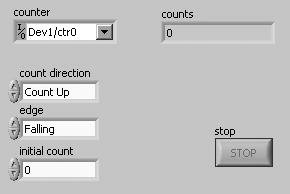
Figure 11.69. Counter measurement types Activity 11-9: Counting Digital PulsesSo, how do you count pulses in LabVIEW? In this exercise, you will see just how simple it is to count pulses with NI-DAQmx in LabVIEW.
For this activity, a simulated NI-DAQmx device will run, but it will not show pulse counts. You will need a physical NI-DAQmx device that has at least one counter channel, in order to count pulses.
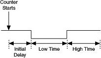
Each time you touch the jumper wire to connect the terminals, you may see hundreds of counts. This is because the connection of the wire touching the terminal is not very good. Digital Pulse Generation with CountersCounters also allow you to generate output signals with the timing characteristics that you definethe same characteristics that a counter can measure, as just described. Table 11.4 contains the basic setup parameters for generating signals using your counter, some of which are illustrated in Figure 11.74.
Figure 11.74. Pulse setup parameter illustration You can also specify how many pulses you wish to generate, or whether you want to generate pulses forever (or at least until you stop the NI-DAQmx generation task). This is called the Generation Mode, and the possible options are described in Table 11.5.
Activity 11-10: Generating Digital PulsesExperiment and try to create a VI that generates 1 pulse, another that generates N pulses, and another that generates continuous digital pulses. (Use the Digital Output>>Counter Output task type.) Wire the counter output that you use for this activity into the counter input you used for the last activity, "Counting Digital Pulses," and count the pulses that you generate. |


EAN: 2147483647
Pages: 294
- ERP Systems Impact on Organizations
- Enterprise Application Integration: New Solutions for a Solved Problem or a Challenging Research Field?
- The Effects of an Enterprise Resource Planning System (ERP) Implementation on Job Characteristics – A Study using the Hackman and Oldham Job Characteristics Model
- Data Mining for Business Process Reengineering
- Development of Interactive Web Sites to Enhance Police/Community Relations