B.1 Reducing the Query to a Query Diagram

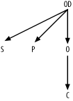
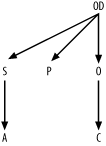
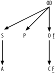
For the first step in the process, create a query diagram. Start with a query skeleton, and then add detail to complete the diagram. The next few subsections walk you through the process of creating the diagram for the example query.

B.1.1 Creating the Query Skeleton

As a starting point, place a random alias in the center of the diagram under construction. For illustration purposes, I'll begin with the node O . Draw arrows downward from that node to any nodes that join to O through their primary key (named, for all these tables, by the same name as the table, with the s at the end replaced by _ID ). Draw a downward-pointing arrow from any alias to O for any join that joins to O on the Orders table's primary key, Order_ID . The beginning of the query skeleton should look like Figure B-1.

Figure B-1. The beginning of the query skeleton

Now, shift focus to OD . Find joins from that node, and add those links to the join skeleton. The result is shown in Figure B-2.

Figure B-2. An intermediate stage of the query skeleton

Find undiagramed join conditions. The only one left is S.Address_ID = A.Address_ID , so add a link for that join to complete the query skeleton, as shown in Figure B-3.

Figure B-3. The completed query skeleton

B.1.2 Creating a Simplified Query Diagram

To build the simplified query diagram, find the most selective filter and identify it with an underlined F next to the filtered node. The condition on the customer's phone number is almost certainly the most selective filter. Add a small underlined f for the only other filter, the much less selective condition on Business_Unit_ID for Orders . The result, shown in Figure B-4, is the simplified query diagram.

Figure B-4. The simplified query diagram

B.1.3 Creating a Full Query Diagram

The simplified query diagram is sufficient to tune this particular query. However, for purposes of illustration, I will show the creation of a full query diagram, with all the details. Use the following queries to gather statistics necessary for a full query diagram. The results I'm using for this example are shown following each query. As an exercise, you might wish to work out the filter and join ratios for yourself.

  Q1:  SELECT SUM(COUNT(Phone_Number)*COUNT(Phone_Number))/   (SUM(COUNT(Phone_Number))*SUM(COUNT(*))) A1   FROM Customers   GROUP BY Phone_Number;  A1:  0.000003  Q2:  SELECT COUNT(*) A2 FROM Customers;  A2:  500,000  Q3:  SELECT SUM(COUNT(Business_Unit_ID)*COUNT(Business_Unit_ID))/   (SUM(COUNT(Business_Unit_ID))*SUM(COUNT(*))) A3   FROM Orders   GROUP BY Business_Unit_ID;  A3:  0.2  Q4:  SELECT COUNT(*) A4 FROM Orders;  A4:  400,000  Q5:  SELECT COUNT(*) A5   FROM Orders O, Customers C   WHERE O.Customer_ID = C.Customer_ID;  A5:  400,000  Q6:  SELECT COUNT(*) A6 FROM Order_Details;  A6:  1,200,000  Q7:  SELECT COUNT(*) A7   FROM Orders O, Order_Details OD   WHERE OD.Order_ID = O.Order_ID;  A7:  1,2000,000  Q8:  SELECT COUNT(*) A8 FROM Shipments;  A8:  540,000  Q9:  SELECT COUNT(*) A9   FROM Shipments S, Order_Details OD   WHERE OD.Shipment_ID = S.Shipment_ID;  A9:  1,080,000  Q10: SELECT COUNT(*) A10 FROM Products;  A10: 12,000  Q11: SELECT COUNT(*) A11   FROM Products P, Order_Details OD   WHERE OD.Product_ID = P.Product_ID;  A11: 1,200,000  Q12: SELECT COUNT(*) A12 FROM Addresses;  A12: 135,000  Q13: SELECT COUNT(*) A13   FROM Addresses A, Shipments S   WHERE S.Address_ID = A.Address_ID;  A13: 540,000 

I downsized the tables in this example so that I could provide practical data-generation scripts to test the execution plans that cost-based optimizers will generate for these tables. If you want to follow along with the example, you can download these scripts from the O'Reilly catalog page for this book: http://www.oreilly.com/catalog/sqltuning/. (However, I cannot guarantee identical results, since results depend on your database version number, parameters set by your DBA, and the data.) The larger tables in this example would likely be around 10 times bigger in a production environment.

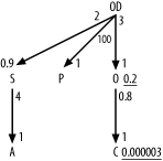
Beginning with filter ratios, get the weighted-average filter ratio for the condition on Customers Phone_Number directly from A1 , which is the result from query Q1 (0.000003). Find the filter ratio on Orders the same way, from Q3 , which returns the result of 0.2 for A3 .

Since no other alias has any filters, the filter ratios on the other four are 1.0, which you imply by just leaving filter ratios off the query diagram for the other nodes.

For each join, find the detail join ratio, to place alongside the upper end of each join arrow, by dividing the count on the join of the two tables by the count on the lower table (the master table of that master-detail relationship). The ratios for the upper ends of the joins from OD to S , O , and P are 2 ( A9 / A8 ), 3 ( A7 / A4 ), and 100 ( A11 / A10 ), respectively. The ratio for the upper end of the join from S to A is 4 ( A13 / A12 ). The ratio for the upper ends of the join from O to C is 0.8 ( A5 / A2 ).

Find the master join ratios, to place alongside the lower end of each join arrow, by dividing the count on the join of the two tables by the count on each upper table (the detail table of a master-detail relationship). The ratio for the lower end of the join from OD to S is 0.9 ( A9 / A6 ). All the other master join ratios turn out to be 1.0, so leave these off the diagram.

Add filter ratios and join ratios to the query skeleton (see Figure B-3) to create the full query diagram, as shown in Figure B-5.

Figure B-5. The full query diagram