DATA MINING
| only for RuBoard - do not distribute or recompile |
DATA MINING
Data mining has a kind of magical reputation. Simply by pointing a data mining tool at a database reveals intriguing and unlikely patterns of behavior. There is folklore building up regarding the serendipitous nature of data mining. The reality is that, while data mining can indeed uncover hitherto unknown relationships in the data, there is nothing serendipitous about it at all. It is a systematic, interactive, and iterative process. For its success it relies on the business expertise of those interpreting the results of its analysis. An apparently useless pattern in the data can be transformed into valuable information if the right business interpretation can be applied. Conversely, a seemingly significant relationship can be explained and disregarded when business experience and commercial knowledge are used.
There are two principal types of data mining:
Hypothesis verification. This is where we might have some idea or hunch about the significance of a relationship between data elements. For instance, someone working in the marketing department of a supermarket retail chain might own a dog. Dogs are notorious for shedding fur in the summer months, and this takes some effort in cleaning up. Therefore, a reasonable hypothesis might be that dog owners will consume more vacuum cleaner bags than the average customer. It might be to the advantage of the company's store managers to place a second rack of vacuum cleaner bags near the dog food. The marketing executive could run some tests to prove (or maybe disprove) this hypothesis.
Knowledge discovery. This is where there may exist hitherto unknown statistically significant relationships between elements of data that no human is likely to deduce. These are the cases that can bring real windfall rewards.
Before embarking upon a mining project and, therefore, investing in an expensive data mining product, it is worth just reviewing whether or not we are likely to be getting some value out of it. First, in order to do data mining, the one thing we absolutely do need is data. Another issue is that the data has to be of good quality and it really should be properly integrated. One of the problems encountered in data mining is poor-quality data, and the risk associated with this is that the errors in the data might affect the results of the mining process. This is known as noise in data mining. Some products claim to be able to handle up to 50 percent noise in data. Nevertheless, the greater the noise, the less accurate the predictions are likely to be. If the data mining exercise forms part of our CRM project, then the most sensible source of data would be the data pool.
Another popular misconception about data mining is that it needs lots and lots of data. This is not true, but what is important is that the data should be truly representative and not skewed one way or another. As long as the range of possible outcomes is covered by the data, good results can be achieved with relatively small volumes .
Some of the major data mining products have evolved from statistical analysis systems and work best with their own proprietary file management systems. Although most now also work with standard ASCII files, it is worth checking that they can also access relational tables. If not, or if they approach it in a very inefficient way, then we might be faced with having to perform expensive extractions and sorts in order to get the data in a form that the data mining product can use. Also, when a vendor says their system can read ASCII files, just check whether they mean fixed length records, comma delimited records, etc. One other thing, if we are allowed to change the field delimiter from comma to something else, that would be very useful. Comma delimiters are fine so long as our fields don't naturally contain commas (e.g., in addresses and in numeric values).
Here are some of the features of data mining products:
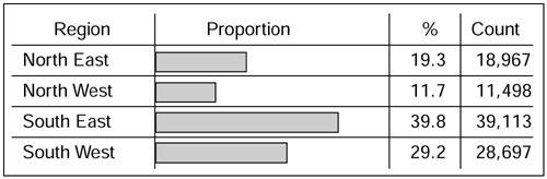
Distributions. How data values are distributed across the value domain is an analysis that is performed very often in statistics. There is a slight difference in the ways in which numeric data is analyzed as opposed to descriptive data. A simple distribution using descriptive information would be between, say, males and females or between geographical regions . The analysis of descriptive data tends to result in a distribution based on absolute set values, as the chart in Figure 10.3 shows.
Figure 10.3. Descriptive field distribution.
Due to the wide range of numeric values, it is not appropriate to use a set-based distribution chart such as the one in Figure 10.3 because it might end up being several hundred pages long. Having said that we could, of course, imagine an analysis based on a descriptive field that also could end up being very long. We might, if we were daft enough, conduct an analysis on, say, address. Unfortunately, these systems won't prevent us from doing silly things.
Anyway, with respect to numeric fields, there are a couple of techniques that are common and should be supported by most products. The first of these is the histogram distribution, which is shown in Figure 10.4.
Figure 10.4. Numeric field distribution using a histogram.
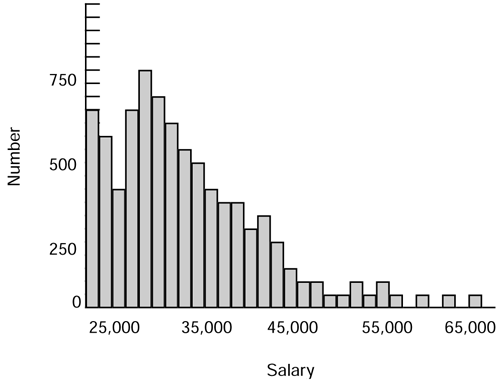
The histogram shows the number of people enjoying salaries at a particular level. In practice, each vertical bar on the chart represents a range of salaries.
The other main type of distribution for numeric data is just referred to as statistics. This gives a more detailed analysis of numeric fields such as the mean, standard deviation, etc., but it does not give as detailed a distribution as the histogram. Here is an example:
| Statistics for field: Salary | |
|---|---|
| Minimum | 23,998 |
| Maximum | 67,290 |
| Occurrences | 98,276 |
| Mean | 30,010 |
| Standard deviation | 1,774 |
Relationships. When searching for relationships between data, the same issues regarding descriptive and numeric fields apply.
For relating descriptive fields to other descriptive fields, it is common to produce a kind of cross-tabulation matrix. Table 10.1 is an example.
Table 10.1. Example of a Field Matrix
Males % Females % North East 17.67 16.22 North West 22.12 21.87 South East 41.23 40.55 South West 18.98 21.66 Notice that, in this example, the percentages add up down the column showing the spread of the genders across region. Some products enable this to be switched around so that we could see the percentages adding to 100 across the rows. This would show the spread of males versus females in each region.
Another way of relating descriptive fields together is to use a web plot. A web plot example is shown in Figure 10.5.
Figure 10.5. Web plot that relates gender to regions.
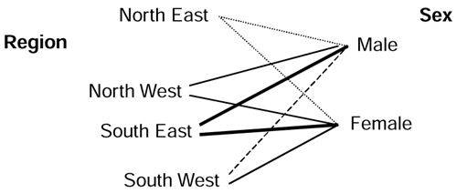
The density of the line between the two nodes indicates the relative strength of the relationship between the two items. The thicker the line, the more significant the relationship.
Apart from histograms, numeric information can also be displayed on scatter plots. The density of the plots indicates the significance of the relationship between the data elements.
Neural networks. The neural network attempts to emulate the human brain, albeit in a very simplistic fashion. In a nutshell , this is how we use them: First, we should present the system with a set of data where the outcome is already known. Let's say that we want to focus our sales effort on a particular wine in the Wine Club catalog. One way to do this is to select out of the data warehouse a set of customers' details, behavior, and circumstances, of customers including some who have already purchased this wine. Now we present this data to the data mining system. We have to tell it what it is we are trying to do, insofar as there needs to be an indicator such as Bought the Wine, yes or no. We also have to tell the system that this indicator is our target, the field that we will be asking it to predict. The data mining system then builds a neural network. It does this by relating every input field to every other input field. By repeatedly relating fields together and calculating weightings for each field, the system builds up a profile and makes a prediction. The prediction is compared to the actual result and, if it is within a predefined tolerance, the process is finished; otherwise the system keeps trying. The system should provide the facility for us to intervene and set its weightings to help it along. If we think we know that a particular field is more relevant than others, then we can increase the weighting . An example might be that the wine is quite expensive and so a customer's salary is likely to be a significant field. Similarly, we don't want the system wasting too much time on low influencing factors, such as, say, the customers' hobbies.
Once the system has learned the relationships within the data, we present it with another set of data where we know the outcome but it doesn't. We can then compare its predictions with what happened in real life. If it is sufficiently accurate for our requirements, we can proceed to the next stage. If not, we return to the previous stage.
When the system has come up with an acceptable level of successful prediction, we can apply the predictive algorithm to the unseen data. Unlike the data that is used to train and test the system, with unseen data the outcome is not known. If the training has been successful, this should result in a list of customers who have a high likelihood of wanting to purchase this product.
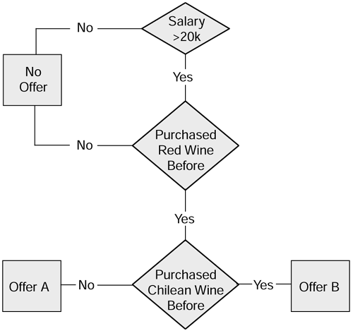
Rule induction. The rule induction technique is very much simpler than neural networks and works on the principle of a predefined set of decision points known as rules. In reality they are like a complex decision tree where you start at the top with a question and, depending on the answer, traverse one of the branches to the next level and another question, and so on. The important thing to remember here is that the rules have to be defined by people with extensive business knowledge. The purpose of the rules-based approach is to attempt to emulate, electronically , the decision behavior of business experts. A simple example of rule induction is shown on Figure 10.6.
Figure 10.6. Rule induction for wine sales.
Another thing to remember about predictive models is that, where possible, we should always try to use more than one so that, in effect, they corroborate each other's predictions. So, when choosing a data mining product, it is probably worth selecting one that has a reasonably wide range of functions.
| only for RuBoard - do not distribute or recompile |
EAN: 2147483647
Pages: 96
- The Second Wave ERP Market: An Australian Viewpoint
- The Effects of an Enterprise Resource Planning System (ERP) Implementation on Job Characteristics – A Study using the Hackman and Oldham Job Characteristics Model
- Context Management of ERP Processes in Virtual Communities
- Healthcare Information: From Administrative to Practice Databases
- A Hybrid Clustering Technique to Improve Patient Data Quality