BUILDING A DATA WAREHOUSE

only for RuBoard - do not distribute or recompile

BUILDING A DATA WAREHOUSE

Now that the Wine Club has decided to build a data warehouse, it must further decide:

1. Where is it to be placed?

2. What technology should be used?

3. How will it be populated ?

These are problems experienced by most organizations when they attempt to build a data warehouse. As we have said, the business applications have been designed using technology and methodologies that were appropriate when they were developed. At the time, no consideration was given to decision support. The applications were designed to satisfy the business operational requirements.

The Wine Club must draw its warehouse data from three very different software environments:

1. Indexed sequential

2. RDBMS

3. Third-party package

Also, these applications reside on two very different hardware platforms (PCs and mid-range computers). The question is:

Are any of the current hardware/software environments appropriate for the data warehouse (in particular, could the data warehouse be kept in an existing database), or should they introduce another set of technologies?

Usually, the warehouse is developed separately from any other application, in a database of its own. One obvious reason for this is, as stated above, due to the disparate nature of the source systems. There are other reasons, however:

1. There is a conflict between operational systems and data warehouse systems in that operational systems are organized around operational requirements and are not subject oriented.

2. Operational systems are constantly changing, whereas decision support systems are quiet (nonvolatile).

3. Operational systems schemas are often very large and complex, where any two tables might have multiple join paths. These complex relationships exist because the business processes require them. It follows that a knowledge worker writing queries has more than one option when attempting to join two tables. Each possible join path will produce a different result. The decision support schema allows only one join path .

An example may help to explain this. Have a look at the entity relationship diagram in Figure 2.4. The example is deliberately unrealistic in order to illustrate the point. The question we have been asked by the directors is:

Which products are more popular in the Northwest?

This is a perfectly reasonable question. But how do we answer it? Assuming the data is stored in a relational database, we have to construct an SQL query that joins the Area table to the Product table in some way.

Figure 2.4. Data model showing multiple join paths.

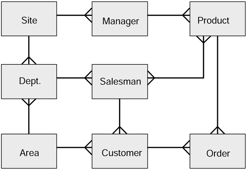
Consider the following questions:

1. How many join paths are there between area and product?

2. Which is the most appropriate?

3. If six people were asked to answer this question, would they always choose the same path?

4. Will all the join paths produce the same result?

The first three questions are kind of rhetorical . The answer to question four is no. For instance, if any of the tables contains no rows, then any join path including that table will not return any rows. So how does the decision maker know that the result is correct?

Another reason for keeping the systems separate is that operational systems do not normally hold historical data. While this is a design issue and, clearly, these systems could hold such data, the effect on performance is not likely to be acceptable to the operational system users. It is usually acceptable for a strategic question to take several minutes, or even hours, to be answered . It would not usually be acceptable for operational system updates to take more than a few seconds.

In any case, most applications that use the database are not developed with historical reporting in mind. This means that, in order to introduce time variance, the applications would have to be modified, sometimes quite substantially. It is usually the case that organizations would not be prepared to tolerate the disruption this would cause. We will be exploring the issues surrounding time in very great detail in Chapter 4.

To answer the question about which is the best technology upon which to build a data warehouse, the RDBMS has emerged as a de facto standard.

Part of the reason for this is that, as we have shown, data warehouses are usually designed using dimensional modeling and the relational model supports the dimensional model very well. This is something we will review in Chapter 3.

There are several components to a data warehouse. Some are concerned with getting the information out of the source systems and into the warehouse, while others are concerned with getting the information out of the warehouse and presenting it to the users.

Figure 2.5 shows the main components.

Figure 2.5. The main components of a data warehouse system.

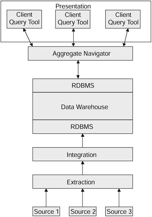
We now examine each of the components of the warehouse model, starting from the bottom.

The Extraction Component

We have established that the subject area for our Wine Club data warehouse is sales and we know that we wish to analyze sales by product, customer, area and, of course, time.

The first problem is to extract information about sales from the source systems so that the sales can be inserted into the warehouse.

In order to insert details about sales into the warehouse, we must have a mechanism for identifying a sale. Having identified the sale, it must be captured and stored so that it may be placed into the warehouse at the appropriate time.

Care must be taken to ensure what is meant by the term sale. If you look carefully at the original EAR model for the Wine Club, you will see that there is no attribute in the system that in any way refers to sales. This is a common problem in data warehouse developments.

Clearly, the Wine Club does sell things. So how do we identify when a sale has occurred? The answer is ”we ask.

The question What is a sale? has to be asked and a definition of sale must be clearly stated and agreed on by everyone before the data can be extracted. You will find that there are usually several different views and each is equally valid, such as:

• A salesperson will normally consider that a sale has occurred when the order has been received from a customer.

• A stock manager will record a sale upon receipt of a notice to ship an order.

• An accountant doesn't usually recognize a sale until an invoice has been raised against an order, usually after it has been shipped.

Although these views are different, there is a common thread, which is that they are all related to the Order entity. What happens is that customers' orders, like all entities, have a lifecycle. At each stage in its lifecycle, the order has a status and a typical order moves logically from one status to the next until its lifecycle is complete and it is removed from the system.

The three different views of a sale, described above, are simply focusing on different states of the same entity (the order).

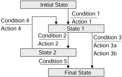
This problem can usually be solved by constructing a state transition diagram, which traces the lifecycle of the entity and defines the events that enable the entity to move from one logical state to the next logical state.

Figure 2.6 shows the general form of a state transition diagram. Note that, although the diagram shows four states and five transitions, in practice there are no limits to the numbers of states or transitions.

Figure 2.6. General state transition diagram.

The state transition diagram for an order in the Wine Club is shown in Figure 2.7.

Figure 2.7. State transition diagram for the orders process.

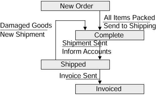
The Wine Club directors have decided that a sale occurs when an order is shipped to a customer. This means that whenever an order changes its status from complete to shipped, that is the point at which the order must be recorded for subsequent insertion into the data warehouse. The only way to achieve this is to make some change to the application so that the change in status is recognized and captured.

Most organizations are not prepared to consider redeveloping their operational systems in order to introduce a data warehouse. Instead, the application software has to be modified to capture the required data into temporary stores so that they may be placed into the warehouse subsequently.

In the case of third-generation language (3GL) based applications such as the Wine Club's order processing and shipment systems, the changes are implemented by altering the programs so that they create temporary data stores as, say, sequential files.

As you may know, relational database management systems often provide the capability for triggers to be stored in the database. These triggers are table-related SQL statements that are executed (sometimes expressed as fired , hence the name trigger) each time a row is inserted, updated, or deleted.

We can create triggers to examine the status of an order each time the order is updated. As soon as the status indicates that a sale has occurred, the trigger logic can record the order in a temporary table for subsequent collection into the warehouse.

The use of packaged applications sometimes requires the original developers to become involved to make the required changes so that the data is available to the data warehouse.

The order entity does have a status column. So the application programs are altered to add a record (for each order item) into a temporary sequential file each time an order changes its status from complete to shipped. The data to be stored are as follows:

• Customer code

• Wine code

• Order date

• Ship date

• Quantity

• Item cost

Every order is captured when, and only when, its status changes from completed to shipped.

That completes the extraction of the sales information. It is not, however, the end of the extraction process.

We still have to extract the information relating to the dimensions of analysis, the points of the star in the star schema.

The customer information is held in a relational database. So obtaining an initial file of customers is a relatively straightforward exercise. The tables in question would be copied to a file using the RDBMS's export utility program. Obtaining details of new customers and changes to existing customers is slightly more tricky but is probably best accomplished by the use of database triggers as described above. Each time a customer's details are updated, the update trigger is fired and we can record the change (sometimes called the delta) into a sequential file for subsequent transfer into the warehouse.

You might be wondering, at this point, why we are bothering to do this at all. You may be thinking that there is a perfectly usable customers' table sitting in the database already. Phrases like unnecessary and uncontrolled duplication of data, that is, data redundancy, may well be coming to mind. These are perfectly correct and reasonable concerns and we will address them shortly.

Similarly, we have not discussed the capture of, and actions for, deleting customers' details. See if you can work out why. If not, don't worry because we will be coming to that later as well.

We also need to capture information relating to products. This is all held on PCs within a third-party software product. Extracting this information can vary from trivial to impossible depending on the quality of the software and the attitude of the software company involved. Usually, some arrangement can be made whereby the software company either alters its product or provides us with sufficient information so that we can write some additional programs to capture the data we need.

Lastly we need information about Areas. Recall that one of the dimensions of analysis is the area in which the customers live. There is no such attribute in the system at present. Therefore, some additional work will be needed to obtain this information.

There are a number of outside agencies that specialize in providing geographic and demographic information. Their customers are often market research organizations and insurance companies that make heavy use of such statistics. So the Wine Club could obtain the information from outside.

Alternatively, another program could be written to process the customers' addresses and analyze them into major towns, or counties or post code groups, etc.

The extraction part of the data warehouse is now complete.

The Integration Component

Some of the issues relating to integration were described in the definition of data warehouses. There are, in fact, two main aspects of integration:

1. Format integration

2. Semantic integration

Format Integration

The issue of format integration is concerned mainly with ensuring that domain integrity is restored where it has been lost. In most organizations, there are usually many cases where attributes in one system have different formats to the same, or similar attributes in other systems. For example:

• Bank account numbers or telephone numbers might be stored as type String in one system and type Numeric in others.

• Sex might be stored as male, / female , m / f, M / F or even 1,0.

• Dates, as previously described can be held in many formats including ddmmyy, ddmmyyyy, yymmdd, yyyymmdd, dd mon yy, dd mon yyyy. These are just a few examples. Some systems store dates as a time stamp that is accurate to thousandths of a second. Others use an integer that is the number of seconds from a particular time, for example, 1 Jan 1900.

• Monetary attributes are also a problem. Some systems store money as integer values and expect the application to insert the decimal points. Others have embedded decimal places.

• In different systems, differing sizes are used for string values such as names , addresses, and product descriptions, etc.

Format integration mismatches are very common, and this is especially true when data is extracted from systems where any of the following is true:

1. The underlying hardware is different.

2. The operating system is different.

3. The application software is different.

The integration procedure consists of a series of rules that are designed to ensure that the data that is loaded into a data warehouse is standardized. So all the dates are the same format, monetary values are always represented the same way, etc.

Why is this important?

Imagine you are attempting to use the data warehouse and you want a list of all employees grouped by sex, age, and average salary where none of those attributes were properly standardized.

It would be a difficult enough task for an experienced programmer to undertake. It would be next to impossible for a non-IT person.

Also, a data warehouse accepts information from a variety of sources into a single table. This is feasible only if the data is of a consistent type and format.

The integration rule set is used as a kind of map that specifies how information that has been extracted from the source systems has to be converted before it is allowed into the data warehouse.

Semantic Integration

As you know, semantics concerns the meaning of data. Data warehouses draw their data from many different operational systems. Typically, different operational systems are used by different people in an organization. This is logical since financial systems are most likely to be used by the accounts department, whereas stock control systems will be used by warehouse (real warehouse, not data warehouse) staff.

Think back to the discussion we had about what a sale is? This kind of ambiguity exists in all organizations and can be very confusing to a database analyst trying to understand the kinds of information being held in systems. The problem is compounded because, often, the users of the systems and the information are unaware of the problem. In everyday conversations, the fact that they are unknowingly discussing different things may not be obvious to them, and most of the time there are no serious repercussions .

In building a data warehouse, we do not have the luxury of being able to ignore these usually subtle differences in semantics because the information produced by the queries that exercise the data warehouse will be used to support decision making at the highest levels in the organization.

It is vital , therefore, that each item of data that is inserted into the warehouse has a precise meaning that is understood by everyone. To this end, a data warehouse must provide a catalog of information that precisely describes each attribute in the warehouse. The catalog is part of the warehouse and is, in fact, a repository of data that describes other data. This data about data is usually referred to as metadata. The subject of metadata is important and is described in more detail later on.

The Warehouse Database

Once the information has been extracted and integrated, it can be inserted into the data warehouse. The idea is that each day, the information for that day is added to the previous data, thereby extending the history by another day. For anyone looking at the database, it is rather like an archaeologist standing on the beach next to a cliff face. The strata that you can see reflect layers of time covering perhaps millions of years , with each layer having its own story to tell. The data in the data warehouse is built up over time in much the same way. Each layer is a reflection of the organization at a particular point in time.

So how do we actually design the data warehouse database?

The dimensional data model used to describe the data requirements was the star schema. Previously I said that the dimensional model was well supported by the relational model. We can create a relational schema that directly reflects the star schema.

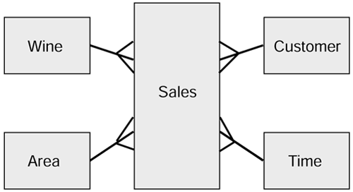
The center of the star schema becomes a relational table, as does each of the dimensions of analysis. The center table is called the fact table because it contains all the facts (i.e., the sales) over which most of the queries will be executed. The dimensions become, simply, dimension tables.

The star schema could be interpreted as several tables (the dimensions) each having a one-to-many relationship with the fact table. We can take the original star schema and attach the crows feet to show this, as in Figure 2.8.

Figure 2.8. Star schema showing the relationships between facts and dimensions.

Entity Descriptions

Sales (CustomerCode, WineCode, OrderTimeCode, AreaCode, Quantity, ItemCost)

Customer ( CustomerCode, CustomerName, CustomerAddress )

Wine ( WineCode, Name, Vintage, ABV, PricePerBottle, PricePerCase)

Area ( AreaCode, AreaDescription)

Time ( TimeStamp, Date, PeriodNumber, QuarterNumber, Year)

Before we continue, it is worth explaining a few things about the diagram.

1. There is no need to record the relationships and their descriptions. In a star schema there is an implicit relationship between the facts and each of the dimensions.

2. The logical identifier of the facts is a composite identifier comprising all the identifiers of the dimensions.

3. Notice the introduction of a time dimension table. The reasoning behind this is connected with the previous point about access to the fact table being driven from the dimension tables.

There are some special characteristics about the kind of data held in the fact table. We have described the primary-key attributes, but what about the non -primary-key attributes: Quantity and Item_Cost. These are the real facts in the fact table. We'll now explore this in more detail.

Figure 2.9 shows the stratified nature of the data as described previously.

Figure 2.9. Stratification of the data.

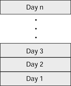
You can visualize lots and lots of rows each containing the composite key, a quantity, and item cost.

How many rows will there be?

Well, according to the original description, the data volumes are:

Over 10 years, allowing for 10 percent growth per annum, the fact table would contain some 62 million rows! Although this is not large in data warehousing terms, it is still a sizable amount of data.

The point is, individual rows in themselves are not very meaningful in a system that is designed to answer strategic questions. In order to get meaningful information about trends, etc., the database needs to be able, as we've said before, to answer questions about sales over time. For instance, to obtain the report analyzing sales by product, the individual sales for a particular product have to be added together to form a total for the product. This means that most queries will need to access hundreds, thousands, or even millions of rows.

What this means, in effect, is that the data in the fact table or, more precisely, the facts in the fact table (Quantity and ItemCost) will almost always have some kind of set function applied to them.

Which of the standard column functions do you think will be the most heavily used in SQL queries against the fact table?

The answer is: the sum function. Almost all queries will use the summation function.

Let's look once more at those famous five questions and see whether our data warehouse can answer them.

Note that questions posed by the users of the data warehouse must usually be interpreted before they can be translated into an SQL query.

Question 1: Which product lines are increasing in popularity and which are decreasing ?

 Select Name,PeriodNumber, sum(Quantity)      From Sales S,Wine W,Time T      Where S.WineCode = W.WineCode      And S.OrderTimeCode = T.TimeCode      And T.PeriodNumber Between 012001 and 122002      Group by Name,PeriodNumber      Order by Name,PeriodNumber 

This query will result in a list of products, each line will show the name, the period, and total quantity sold for that period. If the result set were to be placed into a graph, the products that were increasing and decreasing in popularity would be clearly visible.

Question 2: Which product lines are seasonal?

 Select Name, QuarterNumber, sum(Quantity), sum(ItemCost)      From Sales S, Wine W, Time T      Where S.WineCode = W.WineCode      And S.OrderTimeCode = T.TimeCode      And T.QuarterNumber Between "Q12001" and "Q42002"      Group by Name, QuarterNumber      Order by Name, QuarterNumber 

Question 3: Which customers place the same orders on a regular basis?

This query shows each customer and the name of the wine, where the customer has ordered the same wine more than once:

 Select CustomerName, WineName, Count(*) as "Total Orders"      from Sales S, Customer C, Wine W      Where S.CustomerCode = C.CustomerCode      And S.WineCode = W.WineCode      Group by CustomerName, WineName      Having Count(*) > 1      Order By CustomerName, WineName 

Question 4: Are some products more popular in different parts of the country?

This query shows, for each wine, both the number of orders and the total number of bottles ordered by area.

 Select WineName, AreaDescription,      Count(*) "Total Orders," Sum(Quantity) "Total Bottles"      From Sales S, Wine W, Area A, Time T      Where S.WineCode = W.WineCode      And S.AreaCode = A.AreaCode      And S.OrderTimeCode = T.TimeCode      And T.PeriodNumber Between 012001 and 122002      Group by WineName,AreaDescription      Order by WineName,AreaDescription 

Question 5: Do customers tend to purchase a particular class of product?

This query presents us with a problem. There is no reference to the class of wine in the data warehouse. Information relating to classes does exist in the original EAR model. So it seems that the star schema is incomplete.

What we have to do is extend the Schema as shown in Figure 2.10.

Figure 2.10. Snowflake schema for the sale of wine.

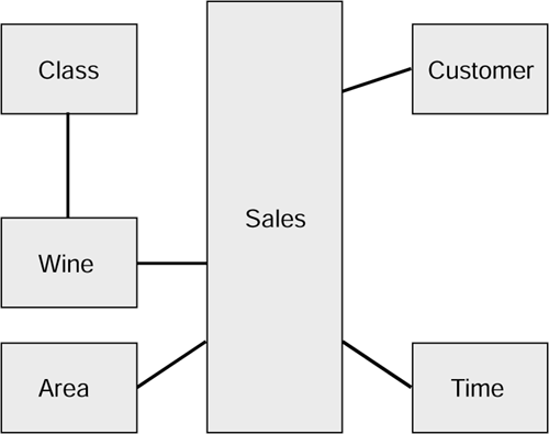
Of course the Class information has to undergo the extraction and integration processing before it can be inserted into the database.

A foreign key constraint must be included in the Wine table to refer to the Class table.

The query can now be coded:

 Select CustomerName, ClassName,             Sum(Quantity) "TotalBottles"      From Sales S,Wine W, Customer Cu, Class Cl, Time T      Where S.WineCode = W.WineCode      And S.CustomerCode = Cu.CustomerCode      And W.ClassCode = Cl.ClassCode      And S.OrderTimeCode = T.TimeCode      And T.PeriodNumber Between 012001 and 122002      Group by CustomerName, ClassName      Having Sum(Quantity) >             2 * (Select AVG(Quantity)                    From Sales S,Wine W, Class C, Time T                    Where S.WineCode = W.WineCode                    And W.ClassCode = C.ClassCode                    And S.OrderTimeCode = T.TimeCode                    And T.PeriodNumber                                   Between 012001 and 122002)      Order by CustomerName, ClassName 

The query lists all customers and classes of wines where the customer has ordered that class of wine at more than twice the quantity as the average for all classes of wine. There are other ways that the query could be phrased. It is always a good idea to ask the directors precisely how they would define their questions in business terms before translating the question into an SQL query.

There are any number of ways the directors can question the data warehouse in order to answer their strategic business questions. We have shown that the data warehouse supports those types of questions in a way in which the operational applications could never hope to do.

The queries show very clearly that the arithmetic functions such as AVG() and particularly SUM() are used in just about every case.

Therefore, a golden rule with respect to fact tables can be defined:

The nonkey columns in the fact table must be summable.

Data attributes such as Quantity and ItemCost are summable, whereas text columns such as descriptions are not summable.

Unfortunately, it is not as straightforward as it seems. Care must be taken to ensure that the summation is meaningful. In some attributes the summation is meaningful only across certain dimensions. For instance, ItemCost can be summed by product, customer, area, and time with meaningful results. Quantity sold can be summed by product but might be regarded as meaningless across other dimensions.

Although this problem applies to the Wine Club, it is much more easily explained in a different organization such as a supermarket . While it is reasonable to sum sales revenue across products (e.g., the revenue from sales of apples added to the revenue from sales of oranges and other fresh fruit each contribute toward the sum of revenue for fresh fruit), adding the quantity of apples sold to the quantity of oranges sold produces a meaningless result.

Attributes that are summable across some dimensions, but not all dimensions, are referred to as semisummable attributes. Clearly they have a valuable role to play in a data warehouse, but their usage must be restricted to avoid the generation of invalid results.

So have we now completed the data warehouse design? Well not quite.

Remember that the fact table may grow to more than 62 million rows over time. There is the possibility, therefore, that a query might have to trawl through every single row of the fact table in order to answer a particular question. In fact, it is very likely that many queries will require a large percentage of the rows, if not the whole table, to be taken into account.

How long will it take to do that? The answer is - quite a long time. Some queries are quite complex, involving multiple join paths, and this will seriously increase the time taken for the result set to be presented back to the user , perhaps to several hours. The problem is exacerbated when several people are using the system at the same time, each with a complex query to run.

If you were to join the 62-million row fact table to the customer table and the wine table, how many rows would the Cartesian product contain?

In principle, there is no need for rapid responses to strategic queries, as they are very different from the kind of day-to-day queries that are executed while someone is hanging on the end of the telephone waiting for a response. In fact, it could be argued that, previously, the answer was impossible to obtain, so even if the query took several days to execute, it would still be worth it.

That doesn't mean we shouldn't do what we can as designers to try to speed things up as much as possible.

Indexes might help, but in a great deal of cases the queries will need to access more than half the data, and indexes are much less efficient in those cases than a full sequential scan of the tables.

No, the answer lies in summaries.

Remember we said that almost all queries would be summing large numbers of rows together and returning a result set with a smaller number of rows. Well if we can predict, to some degree, the types of queries the users will mostly be executing, we can prepare some summarized fact tables so that the users can access those if they happen to satisfy the requirements of the query. Where the aggregates don't supply the required data, then the user can still access the detail.

If we question the users closely enough we should be able to come up with a set, maybe half a dozen or so, of summarized fact tables. The star schema and the snowflake principles still apply, but the result is that we have several fact tables instead of just one.

It should be emphasized that this is a physical design consideration only. Its only purpose is to improve the performance of the queries.

Some examples of summarization for the Wine Club might be:

• Customers by wine for each month

• Customers by wine for each quarter

• Wine by area for each month

• Wine by area for each quarter

Notice that the above examples are summarizing over time. There are other summaries, and you may like to try to think of some, but summarizing over time is a very common practice in data warehouses.

Figure 2.11 shows the levels of summarization commonly in use.

Figure 2.11. Levels of summarization in a data warehouse

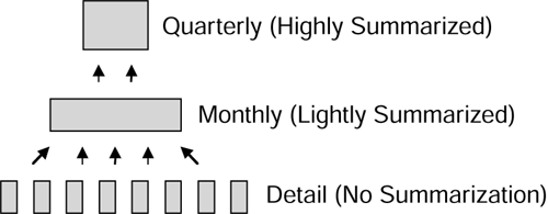
One technique that is very useful to people using the data warehouse is the ability to drill down from one summary level to a lower, more detailed level. For instance, you might observe that a certain range of products was doing particularly well or particularly badly . By drilling down to individual products, you can see whether the whole range or maybe just one isolated product is affected. Conversely, the ability to drill up would enable you to make sure, if you found one product performing badly, that the whole range is not affected.

This ability to drill down and drill up are powerful reporting capabilities provided by a data warehouse where summarization is used.

The usage of the data warehouse must be monitored to ensure that the summaries are being used by the queries that are exercising the database. If it is found that they are not being used, then they should be dropped and replaced by others that are of more use.

Summary Navigation

The introduction of summaries raises some questions:

1. How do users, especially noncomputer professionals, know which summaries are available and how to take advantage of them?

2. How do we monitor which summaries are, in fact, being used?

One solution is to use a summary navigation tool. A summary navigator is an additional layer of software, usually a third-party product, that sits between the user interface (the presentation layer) and the database.

The summary navigator receives the SQL query from the user and examines it to establish which columns are required and the level of summarization needed.

How do summary navigators work?

This is a prime example of the use of metadata. Remember metadata is data about data. Summary navigators hold their own metadata within the data warehouse (or in a database separate from the warehouse).

The metadata is used to provide a mapping between the queries formulated by the users and the data warehouse itself.

Tables 2.2 and 2.3 are example metadata tables.

Summary_Tables

Table  2.2. Available Summary Tables for Aggregate Navigation

Table_Name	DW_Column
Sales_by_Customer_by_Year	Sales
Sales_by_Customer_by_Year	Customer
Sales_by_Customer_by_Year	Year
Sales_by_Customer_by_Quarter	Sales
Sales_by_Customer_by_Quarter	Customer
Sales_by_Customer_by_Quarter	Quarter

Column_Map

Table  2.3. Metadata Mapping Table for Aggregate Navigation

User_Column	User_Value	DW_Column	DW_Value	Rating
Year	2001	Year	2001	100
Year	2001	Quarter	Q1_2001	80
Year	2001	Quarter	Q2_2001	80
Year	2001	Quarter	Q3_2001	80
Year	2001	Quarter	Q4_2001	80

The Summary_Tables table contains a list of all the summaries that exist in the data warehouse, together with the columns contained within them.

The Column_Map table provides a mapping between the columns specified in the user's query and the columns that are available from the warehouse.

Let's look at an example of how it works.

We will assume that the user wants to see the sum of sales for each customer for 2001.

The simple way to do this is to formulate the following query:

 Select CustomerName, Sum(Sales) "Total Sales"          From Sales S, Customer C, Time T          Where S.CustomerCode = C.CustomerCode          And S.TimeCode = T.TimeCode          And T.Year = 2001          Group By C.CustomerName 

As we know, this query would look at every row in the detailed Sales fact table in order to produce the result set and would very likely take a long time to execute.

If, on the other hand, the summary navigator stepped in and grabbed the query before it was passed through to the RDBMS, it could redirect the query to the summary table called Sales_by_Customer_by_Year. It does this by:

1. Checking that all the columns needed are present in the summary table. Note that this includes columns in the Where clause that are not necessarily required in the result set (such as Year in this case).

2. Checking whether there is a translation to be done between what the user has typed and what the summary is expecting.

In this particular case, no translation was necessary, because the summary table Sales_by_Customer_by_Year contained all the necessary columns. So the resultant query would be:

 Select CustomerName, Sum(Sales) "Total Sales"      From Sales_by_Customer_by_Year S, Customer C      Where S.CustomerCode = C.CustomerCode      And S.Year = 2001      Group By C.CustomerName 

If, however, Sales_by_Customer_by_Year did not exist as an aggregate table (but Sales_by_Customer_by_Quarter did) then the summary navigator would have more work to do. It would see that Sales by Customer was available and would have to refer to the Column_Map table to see if the Year column could be derived. The Column_Map table shows that, when the user types Year = 2001, this can be translated to:

 Quarter in ("Q1_2001," "Q2_2001," "Q3_2001," "Q4_2001") 

So, in the absence of Sales_by_Customer_by_Year, the query would be reconstructed as follows:

 Select CustomerName, Sum(Sales) "Total Sales"      From Sales_by_Customer_by_Quarter S, Customer C      Where S.CustomerCode = C.CustomerCode      And S.Quarter in               ("Q1_2001," "Q2_2001," "Q3_2001," "Q4_2001")      Group By C.CustomerName 

Notice that the Column_Map table has a rating column. This tells the summary navigator that Sales_by_Customer_by_Year is summarized to a higher level than Sales_by_Customer_by_Quarter because it has a higher rating. This directs the summary navigator to select the most efficient path to satisfying the query.

You may think that the summary navigator itself adds an overhead to the overall processing time involved in answering queries, and you would be right. Typically, however, the added overhead is in the order of a few seconds, which is a price worth paying for 1000-fold improvements in performance that can be achieved using this technique.

We opened this section with two questions.

The first question asked how users, especially noncomputer professionals, know which aggregates are available and how to take advantage of them.

It is interesting to note that where summary navigation is used, the user never knows which fact table their queries are actually using. This means that they don't need to know which summaries are available and how to take advantage of them. If Sales_by_Customer_by_Year were to be dropped, the summary navigator would automatically switch to using Sales_by_Customer_by_Quarter.

The second question asked how we monitor which summaries are being used. Again, this is simple when you have summary navigator. As it is formulating the actual queries to be executed against the data warehouse, it knows which summary tables are being used and can record the information.

Not only that, it can record:

• The types of queries that are being run to provide statistics so that new summaries can be built

• Response times

• Which users use the system most frequently

All kinds of useful statistics can be stored.

Where does the summary navigator store this information? In its metadata tables.

As a footnote to summary navigation, it is worth mentioning that several of the major RDBMS vendors have expressed the intention of building summary navigation into their products. This development has been triggered by the enormous growth in data warehousing over the past few years.

Presentation of Information

The final component of a data warehouse is the method of presentation. This is how the warehouse is presented to the users.

Most data warehouse implementations adopt a client-server configuration. The concept of client-server, for our purposes, can be viewed as the separation of the users from the warehouse in that the users will normally be using a personal computer and the data warehouse will reside on a remote host. The connection between the machines is controlled by a computer network.

There are very many client products available for accessing relational databases, many of which you may already be familiar with. Most of these products help the user by using the RDBMS schema tables to generate SQL. Similarly, most have the capability to present the results in various forms such as textual reports , pie charts, scatter diagrams, two- and 3-dimensional bar charts , etc. The choice is enormous. Most products are now available on Web servers so that all the users need is a Web browser to display their information.

There are, however, some specialized analysis techniques that have largely come about since the invention of data warehouses. The presence of large volumes of time-variant data, hitherto unavailable, has allowed the development of a new process called data mining.

In our exploration into data warehousing and the ways in which it helps with decision support, the onus has always been placed on the user of the warehouse to formulate the queries and to spot any patterns in the results. This leads to more searching questions being asked as more information is returned.

Data mining is a technique where the technology does more of the work. The users describe the data to the data mining product by identitying the data types and the ranges of valid values. The data mining product is then launched at the database and, by applying standard pattern recognition algorithms, is able to present details of patterns in the data that the user may not be aware of.

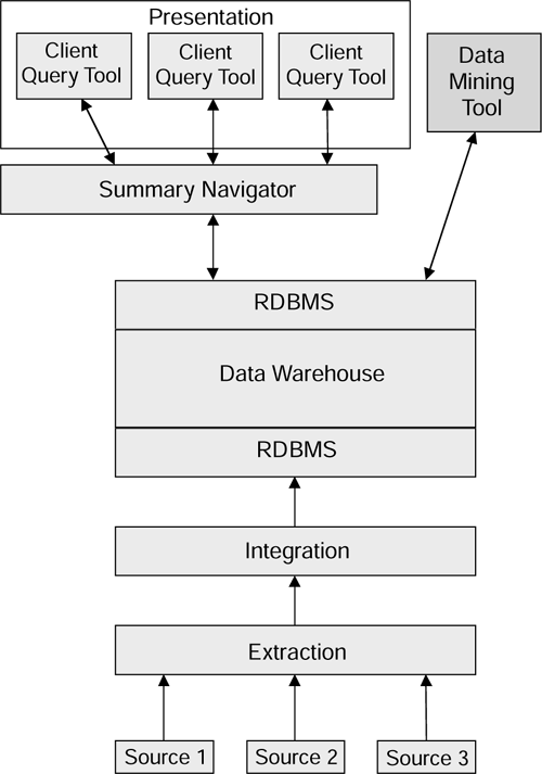
Figure 2.12 shows how a data mining tool fits into the data warehouse model.

Figure 2.12. Modified data warehouse structure incorporating summary navigation and data mining.

The technique has been used very successfully in the insurance industry, where a particular insurance company wanted to decrease the number of proposals for life assurance that had to be referred to the company for approval. A data mining program was applied to the data warehouse and reported that men between the ages of 30 and 40 whose height to weight ratio was within a certain range had an increased risk probability of just 0.015. The company immediately included this profile into their automatic underwriting system, thereby increasing the level of automatic underwriting from 50 percent to 70 percent.

Even with a data warehouse, it would probably have taken a human data miner a long time to spot that pattern because a human would follow logical paths, whereas the data mining program is simply searching for patterns.

only for RuBoard - do not distribute or recompile