Example Problem Solution

[Page 93]

This example demonstrates the transformation of a linear programming model into standard form, sensitivity analysis, computer solution, and shadow prices.

Problem Statement

The Xecko Tool Company is considering bidding on a job for two airplane wing parts . Each wing part must be processed through three manufacturing stagesstamping, drilling, and finishingfor which the company has limited available hours. The linear programming model to determine how many of part 1 ( x ₁ ) and part 2 ( x ₂ ) the company should produce in order to maximize its profit is as follows :

maximize Z = $650 x ₁ + 910 x ₂

subject to

4 x ₁ + 7.5 x ₂ 105 (stamping, hr.)

6.2 x ₁ + 4.9 x ₂ 90 (drilling, hr.)

9.1 x ₁ + 4.1 x ₂ 110 (finishing, hr.)

x ₁ , x ₂

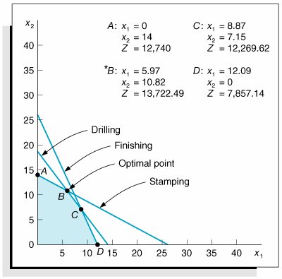
1. Solve the model graphically.

2. Indicate how much slack resource is available at the optimal solution point.

3. Determine the sensitivity ranges for the profit for wing part 1 and the stamping hours available.

4. Solve this model by using Excel.

Solution

1. 

2. The slack at point B , where x ₁ = 5.97 and x ₂ = 10.82, is computed as follows:

   4(5.97) + 7.5(10.82) + s ₁ = 105 (stamping, hr.)

   s ₁ = 0 hr.

   6.2(5.97) + 4.9(10.82) + s ₂ = 90 (drilling, hr.)

   s ₂ = 0 hr.

   9.1(5.97) + 4.1(10.82) + s ₃ = 110 (finishing, hr.)

   s ₃ = 11.35 hr.

   ---

   [Page 94]

3. The sensitivity range for the profit for part 1 is determined by observing the graph of the model and computing how much the slope of the objective function must increase to make the optimal point move from B to C . This is the upper limit of the range and is determined by computing the value of c ₁ that will make the slope of the objective function equal with the slope of the constraint line for drilling, 6.2 x ₁ + 4.9 x ₂ = 90: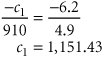

   

   The lower limit is determined by computing the value of c ₁ that will equate the slope of the objective function with the slope of the constraint line for stamping, 4 x ₁ + 7.5 x ₂ = 105:

   

   Summarizing,

   485.33 c ₁ 1,151.43

   The upper limit of the range for stamping hours is determined by first computing the value for q ₁ that would move the solution point from B to where the drilling constraint intersects with the x ₂ axis, where x ₁ = 0 and x ₂ = 18.37: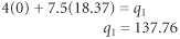

   

   The lower limit of the sensitivity range occurs where the optimal point B moves to C , where x ₁ = 8.87 and x ₂ = 7.15: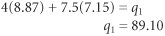

   

   Summarizing, 89.10 q ₁ 137.76.