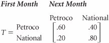
The Transition Matrix

[Page F-5 ( continued )]

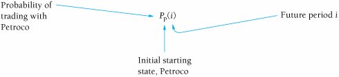
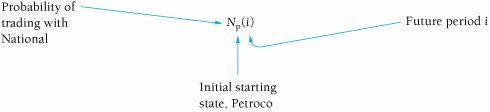
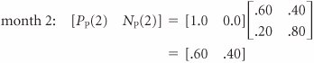
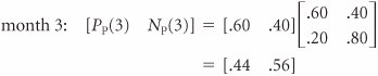
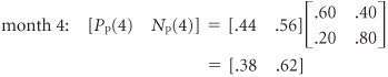
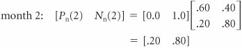
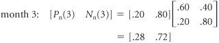
The probabilities of a customer's moving from service station to service station within a 1-month period, presented in tabular form in Table F.1, can also be presented in the form of a rectangular array of numbers called a matrix , as follows :

Because we previously defined these probabilities as transition probabilities, we will refer to the preceding matrix, T , as a transition matrix . The present states of the system are listed on the left of the transition matrix, and the future states in the next time period are listed across the top. For example, there is a .60 probability that a customer who traded with Petroco in month 1 will trade with Petroco in month 2.

A transition matrix includes the transition probabilities for each state of nature.

Several new symbols are needed for Markov analysis using matrix algebra. We will define the probability of a customer's trading with Petroco in period i , given that the customer initially traded with Petroco, as

Similarly, the probability of a customer's trading with National in period i, given that a customer initially traded with Petroco, is

---

[Page F-6]

For example, the probability of a customer's trading at National in month 2, given that the customer initially traded with Petroco, is

N _p (2)

The probabilities of a customer's trading with Petroco and National in a future period, i , given that the customer traded initially with National, are defined as

(When interpreting these symbols, always recall that the subscript refers to the starting state.)

Petroco as the initial starting state.

If a customer is presently trading with Petroco (month 1), the following probabilities exist:

P _p (1) = 1.0

N _p (1) = 0.0

In other words, the probability of a customer's trading at Petroco in month 1, given that the customer trades at Petroco, is 1.0.

These probabilities can also be arranged in matrix form, as follows:

This matrix defines the starting conditions of our example system, given that a customer initially trades at Petroco, as in the decision tree in Figure F.1. In other words, a customer is originally trading with Petroco in month 1. We can determine the subsequent probabilities of a customer's trading at Petroco or National in month 2 by multiplying the preceding matrix by the transition matrix, as follows:

Computing probabilities of a customer trading at either station in future months, using matrix multiplication.

These probabilities of .60 for a customer's trading at Petroco and .40 for a customer's trading at National are the same as those computed in the decision tree in Figure F.1. We use the same procedure for determining the month 3 probabilities, except we now multiply the transition matrix by the month 2 matrix:

These are the same probabilities we computed by using the decision tree analysis in Figure F.1. However, whereas it would be cumbersome to determine additional values by using the decision tree analysis, we can continue to use the matrix approach as we have previously:

---

[Page F-7]

The state probabilities for several subsequent months are as follows:

month 5:	[ P p (5)	N p (5)] = [.35	.65]
month 6:	[ P p (6)	N p (6)] = [.34	.66]
month 7:	[ P p (7)	N p (7)] = [.34	.66]
month 8:	[ P p (8)	N p (8)] = [.33	.67]
month 9:	[ P p (9)	N p (9)] = [.33	.67]

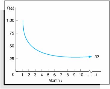
Notice that as we go farther and farther into the future, the changes in the state probabilities become smaller and smaller, until eventually there are no changes at all. At that point every month in the future will have the same probabilities. For this example, the state probabilities that result after some future month, i , are

[ P _p ( i )

N _p ( i )] = [.33

.67]

In future periods, the state probabilities become constant.

This characteristic of the state probabilities approaching a constant value after a number of time periods is shown for P _p ( i ) in Figure F.3.

Figure F.3. The probability P _p (i) for future values of i

N _p ( i ) exhibits this same characteristic as it approaches a value of .67. This is a potentially valuable result for the decision maker. In other words, the service station owner can now conclude that after a certain number of months in the future, there is a .33 probability that the customer will trade with Petroco if the customer initially traded with Petroco.

Computing future state probabilities when the initial starting state is National.

This same type of analysis can be performed given the starting condition in which a customer initially trades with National in month 1. This analysis, shown as follows, corresponds to the decision tree in Figure F.2.

Given that a customer initially trades at the National station, then

[ P _n (1)

N _n (1)] = [0.0

1.0]

Using these initial starting-state probabilities, we can compute future-state probabilities as follows:

---

[Page F-8]

These are the same values obtained by using the decision tree analysis in Figure F.2. Subsequent state probabilities, computed similarly, are shown next:

month 4:	[ P n (4)	N n (4)] = [.31	.69]
month 5:	[ P n (5)	N n (5)] = [.32	.68]
month 6:	[ P n (6)	N n (6)] = [.33	.67]
month 7:	[ P n (7)	N n (7)] = [.33	.67]
month 8:	[ P n (8)	N n (8)] = [.33	.67]
month 9:	[ P n (9)	N n (9)] = [.33	.67]

As in the previous case in which Petroco was the starting state, these state probabilities also become constant after several periods. However, notice that the eventual state probabilities (i.e., .33 and .67) achieved when National is the starting state are exactly the same as the previous state probabilities achieved when Petroco was the starting state. In other words, the probability of ending up in a particular state in the future is not dependent on the starting state.

The probability of ending up in a state in the future is independent of the starting state.