A Mixed Strategy
| A mixed strategy game occurs when each player selects an optimal strategy and the two strategies do not result in an equilibrium point (i.e., the same outcome) when the maximin and minimax decision criteria are applied. A mixed strategy game occurs when each player selects an optimal strategy that does not result in an equilibrium point when the minimax criterion is used . The following example will demonstrate a mixed strategy game. The Coloroid Camera Company (which we will refer to as company I) is going to introduce a new camera into its product line and hopes to capture as large an increase in its market share as possible. In contrast, the Camco Camera Company (which we will refer to as company II) hopes to minimize Coloroid's market share increase. Coloroid and Camco dominate the camera market, and any gain in market share for Coloroid will result in a subsequent identical loss in market share for Camco. The strategies for each company are based on their promotional campaigns , packaging, and cosmetic differences between the products. The payoff table, which includes the strategies and outcomes for each company (I = Coloroid and II = Camco), is shown in Table E.5. The values in Table E.5 are the percentage increases or decreases in market share for company I. Table E.5. Payoff Table for Camera Companies
The first step is to check the payoff table for any dominant strategies. Doing so, we find that strategy 2 dominates strategy 1, and strategy B dominates strategy A. Thus, strategies 1 and A can be eliminated from the payoff table, as shown in Table E.6. Table E.6. Payoff Table with Strategies 1 and A Eliminated
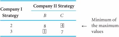
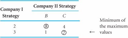
Next, we apply the maximin decision criterion to the strategies for company I, as shown in Table E.7. The minimum value for strategy 2 is 4%, and the minimum value for strategy 3 is 1%. The maximum of these two minimum values is 4%; thus, strategy 2 is optimal for company I. Table E.7. Payoff Table with Maximin Criterion Next, we apply the minimax decision criterion to the strategies for company II in Table E.8. The maximum value for strategy B is 8%, and the maximum value for strategy C is 7%. Of these two maximum values, 7% is the minimum; thus, the optimal strategy for company II is C. Table E.8. Payoff Table with Minimax Criterion Table E.9 combines the results of the application of the maximin and minimax criteria by the companies. Table E.9. Company I and II Combined Strategies
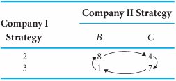
From Table E.9 we can see that the strategies selected by the companies do not result in an equilibrium point. Therefore, this is not a pure strategy game. In fact, this condition will not result in any strategy for either firm. Company I maximizes its market share percentage increase by selecting strategy 2. Company II selects strategy C to minimize company I's market share. However, as soon as company I noticed that company II was using strategy C, it would switch to strategy 3 to increase its market share to 7%. This move would not go unnoticed by company II, which would immediately switch to strategy B to reduce company I's market share to 1%. This action by company II would cause company I to immediately switch to strategy 2 to maximize its market share increase to 8%. Given the action of company I, company II would switch to strategy C to minimize company I's market share increase to 4%. Now you will notice that the two companies are right back where they started. They have completed a closed loop, as shown in Table E.10, which could continue indefinitely if the two companies persisted . In a mixed strategy game, a player switches decisions in response to the decision of the other player and they eventually return to the initial decisions, resulting in a closed loop. Table E.10. Payoff Table with Closed Loop Several methods are available for solving mixed strategy games. We will look at one of them, which is analyticalthe expected gain and loss method . Expected Gain and Loss MethodThe expected gain and loss method is based on the principle that in a mixed strategy game, a plan of strategies can be developed by each player so that the expected gain of the maximizing player or the expected loss of the minimizing player will be the same, regardless of what the opponent does. In other words, a player develops a plan of mixed strategies that will be employed, regardless of what the opposing player does (i.e., the player is indifferent to the opponent 's actions). As might be expected from its name , this method is based on the concept of expected values. In the expected gain and loss method, a plan of strategies is determined by each player so that the expected gain of one equals the expected loss of the other . The mixed strategy game for the two camera companies, described in the previous section, will be used to demonstrate this method. First, we will compute the expected gain for company I. Company I arbitrarily assumes that company II will select strategy B. Given this condition, there is a probability of p that company I will select strategy 2 and a probability of 1 p that company I will select strategy 3. Thus, if company II selects B, the expected gain for company I is 8 p + 1(1 p ) = 1 + 7 p Next, company I assumes that company II will select strategy C. Given strategy C, there is a probability of p that company I will select strategy 2 and a probability of 1 p that company I will select strategy 3. Thus, the expected gain for company I, given strategy C, is 4 p + 7(1 p ) = 7 3 p Previously, we noted that this method was based on the idea that company I would develop a plan that would result in the same expected gain, regardless of the strategy that company II selected. Thus, if company I is indifferent to whether company II selects strategy B or C, we equate the expected gain from each of these strategies: 1 + 7 p = 7 3 p and Recall that p is the probability of using strategy 2, or the percentage of time strategy 2 would be employed. Thus, company I's plan is to use strategy 2 for 60% of the time and to use strategy 3 the remaining 40% of the time. The expected gain (i.e., market share increase for company I) can be computed using the payoff of either strategy B or C because the gain will be the same, regardless. Using the payoffs from strategy B: EG (company I) = .60(8) + .40(1) = 5.2% market share increase To check this result, we compute the expected gain if strategy C is used by company II: EG (company I) = .60(4) + .40(7) = 5.2% market share increase Now we must repeat this process for company II to develop its mixed strategyexcept that what was company I's expected gain is now company II's expected loss . First, we assume that company I will select strategy 2. Thus, company II will employ strategy B for p percent of the time and C the remaining 1 p percent of the time. The expected loss for company II, given strategy 2, is 8 p + 4(1 p ) 4 + 4 p Next, we compute the expected loss for company II, given that company I selects strategy 3: 1 p + 7(1 p ) = 7 6 p Equating these two expected losses for strategies 2 and 3 will result in values for p and 1 p : and 1 p = .70 Because p is the probability of employing strategy B, company II will employ strategy B 30% of the time and, thus, strategy C will be used 70% of the time. The actual expected loss, given strategy 2 (which is the same as that for strategy 3), is computed as The mixed strategies for the two companies are summarized next:
In the expected gain and loss method, the probability that each strategy will be used by each player is computed . The expected gain for company I is a 5.2% increase in market share, and the expected loss for company II is also a 5.2% market share. Thus, the mixed strategies for each company have resulted in an equilibrium point such that a 5.2% expected gain for company I results in a simultaneous 5.2% expected loss for company II. It is also interesting to note that each company has improved its position over the one arrived at using the maximin and minimax strategies. Recall from Table E.4 that the payoff for company I was only a 4% increase in market share, whereas the mixed strategy yields an expected gain of 5.2%. The outcome for company II from the minimax strategy was a 7% loss; however, the mixed strategies show a loss of only 5.2%. Thus, each company puts itself in a better situation by using the mixed strategy approach. This approach assumes that the game is repetitive and will be played over a period of time so that a strategy can be employed a certain percentage of that time. For our example, it can be logically assumed that the marketing of the new camera by company I will require a lengthy time frame. Thus, each company could employ its mixed strategy. The QM for Windows solution of this mixed strategy game for the two camera companies is shown in Exhibit E.2. Exhibit E.2.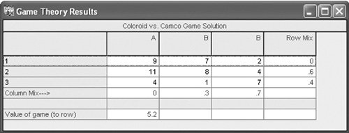 | |||||||||||||||||||||||||||||||||||||||||||||||||||
EAN: 2147483647
Pages: 358