Simplex Solution of a Minimization Problem
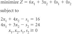
| In the previous section the simplex method for solving linear programming problems was demonstrated for a maximization problem. In general, the steps of the simplex method outlined at the end of this section are used for any type of linear programming problem. However, a minimization problem requires a few changes in the normal simplex process, which we will discuss in this section. In addition, several exceptions to the typical linear programming problem will be presented later in this module. These include problems with mixed constraints (=, Standard Form of a Minimization ModelConsider the following linear programming model for a farmer purchasing fertilizer. where x 1 = bags of Super-gro fertilizer x 2 = bags of Crop-quick fertilizer Z = farmer's total cost ($) of purchasing fertilizer This model is transformed into standard form by subtracting surplus variables from the two The surplus variables represent the extra amount of nitrogen and phosphate that exceeded the minimum requirements specified in the constraints. However, the simplex method requires that the initial basic feasible solution be at the origin, where x 1 = 0 and x 2 = 0. Testing these solution values, we have
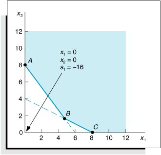
The idea of"negative excess pounds of nitrogen" is illogical and violates the nonnegativityrestriction of linear programming. The reason the surplus variable does not work is shown in Figure A-4. The solution at the origin is outside the feasible solution space. Figure A-4. Graph of the fertilizer example Transforming a model into standard form by subtracting surplus variables will not work in the simplex method. To alleviate this difficulty and get a solution at the origin, we add an artificial variable ( A 1 ) to the constraint equation, 2 x 1 + 4 x 2 s 1 + A 1 = 16 An artificial variable allows for an initial basic feasible solution at the origin, but it has no real meaning. The artificial variable, A 1 , does not have a meaning as a slack variable or a surplus variable does. It is inserted into the equation simply to give a positive solution at the origin; we are artificially creating a solution.
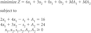
The artificial variable is somewhat analogous to a booster rocket its purpose is to get us off the ground; but once we get started, it has no real use and thus is discarded. The artificial solution helps get the simplex process started, but we do not want it to end up in the optimal solution, because it has no real meaning. When a surplus variable is subtracted and an artificial variable is added, the phosphate constraint becomes 4 x 1 + 3 x 2 s 2 + A 2 = 24 The effect of surplus and artificial variables on the objective function must now be considered . Like a slack variable, a surplus variable has no effect on the objective function in terms of increasing or decreasing cost. For example, a surplus of 24 pounds of nitrogen does not contribute to the cost of the objective function, because the cost is determined solely by the number of bags of fertilizer purchased (i.e., the values of x 1 and x 2 ). Thus, a coefficient of 0 is assigned to each surplus variable in the objective function. By assigning a "cost" of $0 to each surplus variable, we are not prohibiting it from being in the final optimal solution. It would be quite realistic to have a final solution that showed some surplus nitrogen or phosphate. Likewise, assigning a cost of $0 to an artificial variable in the objective function would not prohibit it from being in the final optimal solution. However, if the artificial variable appeared in the solution, it would render the final solution meaningless. Therefore, we must ensure that an artificial variable is not in the final solution. As previously noted, the presence of a particular variable in the final solution is based on its relative profit or cost. For example, if a bag of Super-gro costs $600 instead of $6 and Crop-quick stayed at $3, it is doubtful that the farmer would purchase Super-gro (i.e., x 1 would not be in the solution). Thus, we can prohibit a variable from being in the final solution by assigning it a very large cost . Rather than assigning a dollar cost to an artificial variable, we will assign a value of M , which represents a large positive cost (say, $1,000,000). This operation produces the following objective function for our example: minimize Z = 6 x 1 + 3 x 2 + 0 s 1 + 0 s 2 + MA 1 + MA 2 The completely transformed minimization model can now be summarized as Artificial variables are assigned a large cost in the objective function to eliminate them from the final solution. The Simplex Tableau for a Minimization ProblemThe initial simplex tableau for a minimization model is developed the same way as one for a maximization model, except for one small difference. Rather than computing c j z j in the bottom row of the tableau, we compute z j c j , which represents the net per unit decrease in cost , and the largest positive value is selected as the entering variable and pivot column. (An alternative would be to leave the bottom row as c j z j and select the largest negative value as the pivot column. However, to maintain a consistent rule for selecting the pivot column, we will use z j c j .) The c j z j row is changed to z j c j in the simplex tableau for a minimization problem. The initial simplex tableau for this model is shown in Table A-17. Notice that A 1 and A 2 form the initial solution at the origin, because that was the reason for inserting them in the first place to get a solution at the origin. This is not a basic feasible solution, since the origin is not in the feasible solution area, as shown in Figure A-4. As indicated previously, it is an artificially created solution. However, the simplex process will move toward feasibility in subsequent tableaus. Note that across the top the decision variables are listed first, then surplus variables, and finally artificial variables. Table A-17. The Initial Simplex Tableau
Artificial variables are always included as part of the initial basic feasible solution when they exist. In Table A-17 the x 2 column was selected as the pivot column because 7 M 3 is the largest positive value in the z j c j row. A 1 was selected as the leaving basic variable (and pivot row) because the quotient of 4 for this row was the minimum positive row value. Once an artificial variable is selected as the leaving variable, it will never reenter the tableau, so it can be eliminated. The second simplex tableau is developed using the simplex formulas presented earlier. It is shown in Table A-18. Notice that the A 1 column has been eliminated in the second simplex tableau. Once an artificial variable leaves the basic feasible solution, it will never return because of its high cost, M . Thus, like the booster rocket, it can be eliminated from the tableau. However, artificial variables are the only variables that can be treated this way. Table A-18. The Second Simplex Tableau
The third simplex tableau, with x 1 replacing A 2 , is shown in Table A-19. Both the A 1 and A 2 columns have been eliminated because both variables have left the solution. The x 1 row is selected as the pivot row because it corresponds to the minimum positive ratio of 16. In selecting the pivot row, the 4 value for the x 2 row was not considered because the minimum positive value or zero is selected. Selecting the x 2 row would result in a negative quantity value for s 1 in the fourth tableau, which is not feasible. Table A-19. The Third Simplex Tableau
The fourth simplex tableau, with s 1 replacing x 1 , is shown in Table A-20. Table A-20 is the optimal simplex tableau because the z j c j row contains no positive values. The optimal solution is x 1 = 0 bags of Super-gro s 1 = 16 extra lb of nitrogen x 2 = 8 bags of Crop-quick s 2 = 0 extra lb of phosphate Z = $24, total cost of purchasing fertilizer Table A-20. Optimal Simplex Tableau
Simplex Adjustments for a Minimization ProblemTo summarize, the adjustments necessary to apply the simplex method to a minimization problem are as follows:
Although the fertilizer example model we just used included only |
 , and
, and  ); problems with more than one optimal solution, no feasible solution, or an unbounded solution; problems with a tie for the pivot column; problems with a tie for the pivot row; and problems with constraints with negative quantity values. None of these kinds of problems require changes in the simplex method. They are basically unusual results in individual simplex tableaus that the reader should know how to interpret and work with.
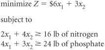
EAN: 2147483647
Pages: 358