The Monte Carlo Process

[Page 612 ( continued )]

One characteristic of some systems that makes them difficult to solve analytically is that they consist of random variables represented by probability distributions. Thus, a large proportion of the applications of simulations are for probabilistic models.

The term Monte Carlo has become synonymous with probabilistic simulation in recent years . However, the Monte Carlo technique can be more narrowly defined as a technique for selecting numbers randomly from a probability distribution (i.e., "sampling") for use in a trial (computer) run of a simulation. The Monte Carlo technique is not a type of simulation model but rather a mathematical process used within a simulation.

Monte Carlo is a technique for selecting numbers randomly from a probability distribution .

The name Monte Carlo is appropriate because the basic principle behind the process is the same as in the operation of a gambling casino in Monaco. In Monaco such devices as roulette wheels, dice, and playing cards are used. These devices produce numbered results at random from well-defined populations. For example, a 7 resulting from thrown dice is a random value from a population of 11 possible numbers (i.e., 2 through 12). This same process is employed, in principle, in the Monte Carlo process used in simulation models.

The Monte Carlo process is analogous to gambling devices .

The Use of Random Numbers

The Monte Carlo process of selecting random numbers according to a probability distribution will be demonstrated using the following example. The manager of Computer-World, a store that sells computers and related equipment, is attempting to determine how many laptop PCs the store should order each week. A primary consideration in this decision is the average number of laptop computers that the store will sell each week and the average weekly revenue generated from the sale of laptop PCs. A laptop sells for $4,300. The number of laptops demanded each week is a random variable (which we will define as x ) that ranges from 0 to 4. From past sales records, the manager has determined the frequency of demand for laptop PCs for the past 100 weeks. From this frequency distribution, a probability distribution of demand can be developed, as shown in Table 14.1.

---

[Page 613]

Table 14.1. Probability distribution of demand for laptop PCs

PCs Demanded per Week	Frequency of Demand	Probability of Demand, P ( x )
	20	.20
1	40	.40
2	20	.20
3	10	.10
4	10	.10
	100	1.00

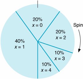
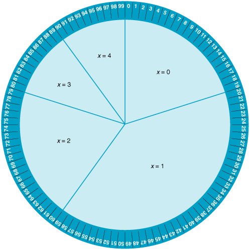
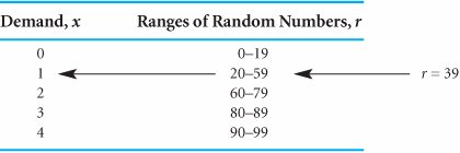
The purpose of the Monte Carlo process is to generate the random variable, demand, by sampling from the probability distribution, P ( x ). The demand per week can be randomly generated according to the probability distribution by spinning a wheel that is partitioned into segments corresponding to the probabilities, as shown in Figure 14.1.

Figure 14.1. A roulette wheel for demand

In the Monte Carlo process, values for a random variable are generated by sampling from a probability distribution .

Because the surface area on the roulette wheel is partitioned according to the probability of each weekly demand value, the wheel replicates the probability distribution for demand if the values of demand occur in a random manner. To simulate demand for 1 week, the manager spins the wheel; the segment at which the wheel stops indicates demand for 1 week. Over a period of weeks (i.e., many spins of the wheel), the frequency with which demand values occur will approximate the probability distribution, P ( x ). This method of generating values of a variable, x , by randomly selecting from the probability distributionthe wheelis the Monte Carlo process.

By spinning the wheel, the manager artificially reconstructs the purchase of PCs during a week. In this reconstruction, a long period of real time (i.e., a number of weeks) is represented by a short period of simulated time (i.e., several spins of the wheel).

A long period of real time is represented by a short period of simulated time .

Now let us slightly reconstruct the roulette wheel. In addition to partitioning the wheel into segments corresponding to the probability of demand, we will put numbers along the outer rim, as on a real roulette wheel. This reconstructed roulette wheel is shown in Figure 14.2.

Figure 14.2. Numbered roulette wheel

(This item is displayed on page 614 in the print version)

There are 100 numbers from 0 to 99 on the outer rim of the wheel, and they have been partitioned according to the probability of each demand value. For example, 20 numbers from 0 to 19 (i.e., 20% of the total 100 numbers) correspond to a demand of no (0) PCs. Now we can determine the value of demand by seeing which number the wheel stops at as well as by looking at the segment of the wheel.

---

[Page 614]

When the manager spins this new wheel, the actual demand for PCs will be determined by a number. For example, if the number 71 comes up on a spin, the demand is 2 PCs per week; the number 30 indicates a demand of 1. Because the manager does not know which number will come up prior to the spin and there is an equal chance of any of the 100 numbers occurring, the numbers occur at random; that is, they are random numbers .

Obviously, it is not generally practical to generate weekly demand for PCs by spinning a wheel. Alternatively, the process of spinning a wheel can be replicated by using random numbers alone.

First, we will transfer the ranges of random numbers for each demand value from the roulette wheel to a table, as in Table 14.2. Next, instead of spinning the wheel to get a random number, we will select a random number from Table 14.3, which is referred to as a random number table . (These random numbers have been generated by computer so that they are all equally likely to occur , just as if we had spun a wheel. The development of random numbers is discussed in more detail later in this chapter.) As an example, let us select the number 39, the first entry in Table 14.3. Looking again at Table 14.2, we can see that the random number 39 falls in the range 2059, which corresponds to a weekly demand of 1 laptop PC.

---

[Page 615]

Table 14.2. Generating demand from random numbers

(This item is displayed on page 614 in the print version)

Table 14.3. Random number table

39 65 76 45 45	19 90 69 64 61	20 26 36 31 62	58 24 97 14 97	95 06 70 99 00
73 71 23 70 90	65 97 60 12 11	31 56 34 19 19	47 83 75 51 33	30 62 38 20 46
72 18 47 33 84	51 67 47 97 19	98 40 07 17 66	23 05 09 51 80	59 78 11 52 49
75 12 25 69 17	17 95 21 78 58	24 33 45 77 48	69 81 84 09 29	93 22 70 45 80
37 17 79 88 74	63 52 06 34 30	01 31 60 10 27	35 07 79 71 53	28 99 52 01 41
02 48 08 16 94	85 53 83 29 95	56 27 09 24 43	21 78 55 09 82	72 61 88 73 61
87 89 15 70 07	37 79 49 12 38	48 13 93 55 96	41 92 45 71 51	09 18 25 58 94
98 18 71 70 15	89 09 39 59 24	00 06 41 41 20	14 36 59 25 47	54 45 17 24 89
10 83 58 07 04	76 62 16 48 68	58 76 17 14 86	59 53 11 52 21	66 04 18 72 87
47 08 56 37 31	71 82 13 50 41	27 55 10 24 92	28 04 67 53 44	95 23 00 84 47
93 90 31 03 07	34 18 04 52 35	74 13 39 35 22	68 95 23 92 35	36 63 70 35 33
21 05 11 47 99	11 20 99 45 18	76 51 94 84 86	13 79 93 37 55	98 16 04 41 67
95 89 94 06 97	27 37 83 28 71	79 57 95 13 91	09 61 87 25 21	56 20 11 32 44
97 18 31 55 73	10 65 81 92 59	77 31 61 95 46	20 44 90 32 64	26 99 76 75 63
69 08 88 86 13	59 71 74 17 32	48 38 75 93 29	73 37 32 04 05	60 82 29 20 25
41 26 10 25 03	87 63 93 95 17	81 83 83 04 49	77 45 85 50 51	79 88 01 97 30
91 47 14 63 62	08 61 74 51 69	92 79 43 89 79	29 18 94 51 23	14 85 11 47 23
80 94 54 18 47	08 52 85 08 40	48 40 35 94 22	72 65 71 08 86	50 03 42 99 36
67 06 77 63 99	89 85 84 46 06	64 71 06 21 66	89 37 20 70 01	61 65 70 22 12
59 72 24 13 75	42 29 72 23 19	06 94 76 10 08	81 30 15 39 14	81 33 17 16 33
63 62 06 34 41	79 53 36 02 95	94 61 09 43 62	20 21 14 68 86	84 95 48 46 45
78 47 23 53 90	79 93 96 38 63	34 85 52 05 09	85 43 01 72 73	14 93 87 81 40
87 68 62 15 43	97 48 72 66 48	53 16 71 13 81	59 97 50 99 52	24 62 20 42 31
47 60 92 10 77	26 97 05 73 51	88 46 38 03 58	72 68 49 29 31	75 70 16 08 24
56 88 87 59 41	06 87 37 78 48	65 88 69 58 39	88 02 84 27 83	85 81 56 39 38
22 17 68 65 84	87 02 22 57 51	68 69 80 95 44	11 29 01 95 80	49 34 35 36 47
19 36 27 59 46	39 77 32 77 09	79 57 92 36 59	89 74 39 82 15	08 58 94 34 74
16 77 23 02 77	28 06 24 25 93	22 45 44 84 11	87 80 61 65 31	09 71 91 74 25
78 43 76 71 61	97 67 63 99 61	30 45 67 93 82	59 73 19 85 23	53 33 65 97 21
03 28 28 26 08	69 30 16 09 05	53 58 47 70 93	66 56 45 65 79	45 56 20 19 47
04 31 17 21 56	33 73 99 19 87	26 72 39 27 67	53 77 57 68 93	60 61 97 22 61
61 06 98 03 91	87 14 77 43 96	43 00 65 98 50	45 60 33 01 07	98 99 46 50 47
23 68 35 26 00	99 53 93 61 28	52 70 05 48 34	56 65 05 61 86	90 92 10 70 80
15 39 25 70 99	93 86 52 77 65	15 33 59 05 28	22 87 26 07 47	86 96 98 29 06
58 71 96 30 24	18 46 23 34 27	85 13 99 24 44	49 18 09 79 49	74 16 32 23 02
93 22 53 64 39	07 10 63 76 35	87 03 04 79 88	08 13 13 85 51	55 34 57 72 69
78 76 58 54 74	92 38 70 96 92	52 06 79 79 45	82 63 18 27 44	69 66 92 19 09
61 81 31 96 82	00 57 25 60 59	46 72 60 18 77	55 66 12 62 11	08 99 55 64 57
42 88 07 10 05	24 98 65 63 21	47 21 61 88 32	27 80 30 21 60	10 92 35 36 12
77 94 30 05 39	28 10 99 00 27	12 73 73 99 12	49 99 57 94 82	96 88 57 17 91

Random numbers are equally likely to occur .

By repeating this process of selecting random numbers from Table 14.3 (starting anywhere in the table and moving in any direction but not repeating the same sequence) and then determining weekly demand from the random number, we can simulate demand for a period of time. For example, Table 14.4 shows demand for a period of 15 consecutive weeks.

---

[Page 616]

Table 14.4. Randomly generated demand for 15 weeks

Week	r	Demand, x	Revenue
1	39	1	$ 4,300
2	73	2	8,600
3	72	2	8,600
4	75	2	8,600
5	37	1	4,300
6	02
7	87	3	12,900
8	98	4	17,200
9	10
10	47	1	4,300
11	93	4	17,200
12	21	1	4,300
13	95	4	17,200
14	97	4	17,200
15	69	2	8,600
		S =31	$133,300

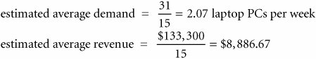
From Table 14.4 the manager can compute the estimated average weekly demand and revenue:

The manager can then use this information to help determine the number of PCs to order each week.

Although this example is convenient for illustrating how simulation works, the average demand could have more appropriately been calculated analytically using the formula for expected value. The expected value or average for weekly demand can be computed analytically from the probability distribution, P ( x ):

where

x i	=	demand value i
P ( x i )	=	probability of demand
n	=	the number of different demand values

Therefore,

E ( x )	=	(.20)(0) + (.40)(1) + (.20)(2) + (.10)(3) + (.10)(4)
	=	1.5 PCs per week

Simulation results will not equal analytical results unless enough trials of the simulation have been conducted to reach steady state .

The analytical result of 1.5 PCs is close to the simulated result of 2.07 PCs, but clearly there is some difference. The margin of difference (0.57 PCs) between the simulated value and the analytical value is a result of the number of periods over which the simulation was conducted. The results of any simulation study are subject to the number of times the simulation occurred (i.e., the number of trials ). Thus, the more periods for which the simulation is conducted, the more accurate the result. For example, if demand were simulated for 1,000 weeks, in all likelihood an average value exactly equal to the analytical value (1.5 laptop PCs per week) would result.

---

[Page 617]

Time Out: For John Von Neumann

The mathematics of the Monte Carlo method have been known for years; the British mathematician Lord Kelvin used the technique in a paper in 1901. However, it was formally identified and given this name by the Hungarian mathematician John Von Neumann while working on the Los Alamos atomic bomb project during World War II. During this project, physicists confronted a problem in determining how far neutrons would travel through various materials (i.e., neutron diffusion in fissile material). The Monte Carlo process was suggested to Von Neumann by a colleague at Los Alamos, Stanislas Ulam, as a means to solve this problemthat is, by selecting random numbers to represent the random actions of neutrons. However, the Monte Carlo method as used in simulation did not gain widespread popularity until the development of the modern electronic computer after the war. Interestingly, this remarkable man, John Von Neumann, is credited with being the key figure in the development of the computer.

Once a simulation has been repeated enough times that it reaches an average result that remains constant, this result is analogous to the steady-state result, a concept we discussed previously in our presentation of queuing. For this example, 1.5 PCs is the long-run average or steady-state result, but we have seen that the simulation might have to be repeated more than 15 times (i.e., weeks) before this result is reached.

Comparing our simulated result with the analytical (expected value) result for this example points out one of the problems that can occur with simulation. It is often difficult to validate the results of a simulation modelthat is, to make sure that the true steady-state average result has been reached. In this case we were able to compare the simulated result with the expected value (which is the true steady-state result), and we found there was a slight difference. We logically deduced that the 15 trials of the simulation were not sufficient to determine the steady-state average. However, simulation most often is employed whenever analytical analysis is not possible (this is one of the reasons that simulation is generally useful). In these cases, there is no analytical standard of comparison, and validation of the results becomes more difficult. We will discuss this problem of validation in more detail later in the chapter.

It is often difficult to validate that the results of a simulation truly replicate reality .