The Normal Distribution
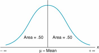
| Previously, a discrete value was defined as a value that is countable (and usually an integer). A random variable is discrete if the values it can equal are finite and countable. The probability distributions we have encountered thus far have been discrete distributions. In other words, the values of the random variables that made up these discrete distributions were always finite (for example, in the preceding example, there were five possible values of the random variable breakdowns per month). Because every value of the random variable had a unique probability of occurrence, the discrete probability distribution consisted of all the (finite) values of a random variable and their associated probabilities. A continuous random variable can take on an infinite number of values within an interval, or range . In contrast, a continuous random variable can take on an infinite number of values within some interval. This is because continuous random variables have values that are not specifically countable and are often fractional . The distinction between discrete and continuous random variables is sometimes made by saying that discrete relates to things that can be counted and continuous relates to things that are measured. For example, a load of oil being transported by tanker may consist of not just 1 million or 2 million barrels but 1.35 million barrels. If the range of the random variable is between 1 million and 2 million barrels, then there is an infinite number of possible (fractional) values between 1 million and 2 million barrels, even though the value 1.35 million corresponds to a discrete value of 1,350,000 barrels of oil. No matter how small an interval exists between two values in the distribution, there is always at least one valueand, in fact, an infinite number of valuesbetween the two values. Because a continuous random variable can take on an extremely large or infinite number of values, assigning a unique probability to every value of the random variable would require an infinite (or very large) number of probabilities, each of which would be infinitely small. Therefore, we cannot assign a unique probability to each value of the continuous random variable, as we did in a discrete probability distribution. In a continuous distribution , we can refer only to the probability that a value of the random variable is within some range . For example, we can determine the probability that between 1.35 million and 1.40 million barrels of oil are transported, or the probability that fewer than or more than 1.35 million barrels are shipped, but we cannot determine the probability that exactly 1.35 million barrels of oil are transported. One of the most frequently used continuous probability distributions is the normal distribution , which is a continuous curve in the shape of a bell (i.e., it is symmetrical). The normal distribution is a popular continuous distribution because it has certain mathematical properties that make it easy to work with, and it is a reasonable approximation of the continuous probability distributions of a number of natural phenomena. Figure 11.8 is an illustration of the normal distribution. Figure 11.8. The normal curve The normal distribution is a continuous probability distribution that is symmetrical on both sides of the meanthat is, it is shaped like a bell . The fact that the normal distribution is a continuous curve reflects the fact that it consists of an infinite or extremely large number of points (on the curve). The bell-shaped curve can be flatter or taller, depending on the degree to which the values of the random variable are dispersed from the center of the distribution. The center of the normal distribution is referred to as the mean ( µ), and it is analogous to the average of the distribution. The center of a normal distribution is its mean, µ . Notice that the two ends (or tails ) of the distribution in Figure 11.8 extend from - The area under the normal curve represents probability, and the total area under the curve sums to one . As an example of the application of the normal distribution, consider the Armor Carpet Store, which sells Super Shag carpet. From several years of sales records, store management has determined that the mean number of yards of Super Shag demanded by customers during a week is 4,200 yards, and the standard deviation is 1,400 yards. It is necessary to know both the mean and the standard deviation to perform a probabilistic analysis using the normal distribution. The store management assumes that the continuous random variable, yards of carpet demanded per week, is normally distributed (i.e., the values of the random variable have approximately the shape of the normal curve). The mean of the normal distribution is represented by the symbol µ, and the standard deviation is represented by the symbol s :
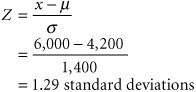
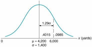
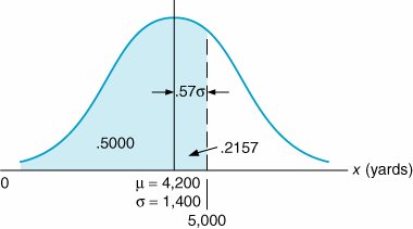
The store manager wants to know the probability that the demand for Super Shag in the upcoming week will exceed 6,000 yards. The normal curve for this example is shown in Figure 11.9. The probability that x (the number of yards of carpet) will be equal to or greater than 6,000 is expressed as Figure 11.9. The normal distribution for carpet demand P ( x which corresponds to the area under the normal curve to the right of the value 6,000 because the area under the curve (in Figure 11.9) represents probability. In a normal distribution, area or probability is measured by determining the number of standard deviations the value of the random variable x is from the mean . The number of standard deviations a value is from the mean is represented by Z and is computed using the formula The area under a normal curve is measured by determining the number of standard deviations the value of a random variable is from the mean . The number of standard deviations a value is from the mean gives us a consistent standard of measure for all normal distributions. In our example, the units of measure are yards; in other problems, the units of measure may be pounds , hours, feet, or tons. By converting these various units of measure into a common measure (number of standard deviations), we create a standard that is the same for all normal distributions. Actually, the standard form of the normal distribution has a mean of zero ( µ = 0) and a standard deviation of one ( s = 1). The value Z enables us to convert this scale of measure into whatever scale our problem requires. Figure 11.10 shows the standard normal distribution , with our example distribution of carpet demand above it. This illustrates the conversion of the scale of measure along the horizontal axis from yards to number of standard deviations. Figure 11.10. The standard normal distribution(This item is displayed on page 495 in the print version) The horizontal axis along the bottom of Figure 11.10 corresponds to the standard normal distribution. Notice that the area under the normal curve between 1 s and 1 s represents 68% of the total area under the normal curve, or a probability of .68. Now look at the horizontal axis corresponding to yards in our example. Given that the standard deviation is 1,400 yards, the area between 1 s (2,800 yards) and 1 s (5,600 yards) is also 68% of the total area under the curve. Thus, if we measure distance along the horizontal axis in terms of the number of standard deviations, we will determine the same probability, no matter what the units of measure are. The formula for Z makes this conversion for us. Returning to our example, recall that the manager of the carpet store wants to know the probability that the demand for Super Shag in the upcoming week will be 6,000 yards or more. Substituting the values x = 6,000, µ = 4,200, and s = 1,400 yards into our formula for Z , we can determine the number of standard deviations the value 6,000 is from the mean: The value x = 6,000 is 1.29 standard deviations from the mean, as shown in Figure 11.11. Figure 11.11. Determination of the Z value The area under the standard normal curve for values of Z has been computed and is displayed in easily accessible normal tables . Table A.1 in Appendix A is such a table. It shows that Z = 1.29 standard deviations corresponds to an area, or probability, of .4015. However, this is the area between µ = 4,200 and x = 6,000 because what was measured was the area within 1.29 standard deviations of the mean. Recall, though, that 50% of the area under the curve lies to the right of the mean. Thus, we can subtract .4015 from .5000 to get the area to the right of x = 6,000: This means that there is a .0985 (or 9.85%) probability that the demand for carpet next week will be 6,000 yards or more. Now suppose that the carpet store manager wishes to consider two additional questions: (1) What is the probability that demand for carpet will be 5,000 yards or less? (2) What is the probability that the demand for carpet will be between 3,000 yards and 5,000 yards? We will consider each of these questions separately. First, we want to determine P ( x Figure 11.12. Normal distribution for P ( x |
 to +
to + 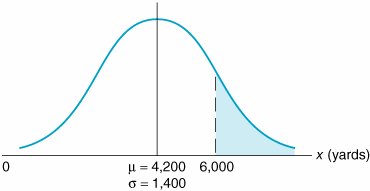
 6,000)
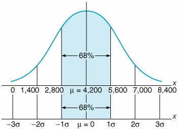
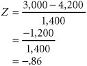
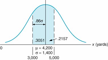
 5,000). The area representing this probability is shown in Figure 11.12. The area to the left of the mean in Figure 11.12 equals .50. That leaves only the area between
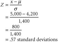

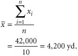
| Week i | Demand x i |
|---|---|
| 1 | 2,900 |
| 2 | 5,400 |
| 3 | 3,100 |
| 4 | 4,700 |
| 5 | 3,800 |
| 6 | 4,300 |
| 7 | 6,800 |
| 8 | 2,900 |
| 9 | 3,600 |
| 10 | 4,500 |
| S = 42,000 |
The sample mean is computed as
The sample variance is computed as
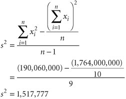
The sample standard deviation, s , is
These values are very close to the mean and standard deviation we originally estimated in this example in the previous section (i.e., µ = 4,200 yd., s = 1,400 yd.). In general, the accuracy of the sample depends on two factors: the sample size ( n ) and the variation in the data. The larger the sample, the more accurate the sample statistics will be in estimating the population statistics. Also, the more variable the data are, the less accurate the sample statistics will be as estimates of the population statistics.
The Chi-Square Test for Normality
Several of the quantitative techniques that are presented in the remainder of this text include probabilistic data and parameters and statistical analysis. In many cases the problem data are assumed (or stated) to be normally distributed, with a mean and standard deviation, which enable statistical analysis to be performed based on the normal distribution. However, in reality it can never be simply assumed that data are normally distributed or in fact reflect any probability distribution. Frequently, a statistical test must be performed to determine the exact distribution (if any) to which the data conform.
The chi-square ( c 2 ) test is one such statistical test to see if observed data fit a particular probability distribution, including the normal distribution. The chi-square test compares the actual frequency distribution for a set of data with a theoretical frequency distribution that would be expected to occur for a specific distribution. This is also referred to as testing the goodness-of-fit of a set of data to a specific probability distribution.
To perform a chi-square goodness-of-fit test, the actual number of frequencies in each class or the range of a frequency distribution is compared to the theoretical frequencies that should occur in each class if the data followed a particular distribution. These numeric differences between the actual and theoretical values in each class are used in a formula to compute a c 2 test statistic, or number, which is then compared to a number from a chi-square table called a critical value . If the computed c 2 test statistic is greater than the tabular critical value, then the data do not follow the distribution being tested ; if the critical value is greater than the computed test statistic, the distribution does exist. In statistical terminology this is referred to as testing the hypothesis that the data are, for example, normally distributed. If the c 2 test statistic is greater than the tabular critical value, the hypothesis (H o ) that the data fits the hypothesized distribution is rejected, and the distribution does not exist; otherwise , it is accepted.
To demonstrate how to apply the chi-square test for a normal distribution, we will use an expanded version of our Armor Carpet Store example used in the previous section. To test the distribution, we need a lot more data than the 10 weeks of demand we used previously. Instead, we will now assume that we have collected a sample of 200 weeks of demand for Super Shag carpet and that these data have been grouped according to the following frequency distribution:
| Range, Weekly Demand (yd.) | Frequency (weeks) |
|---|---|
| 0 < 1,000 | 2 |
| 1,000 < 2,000 | 5 |
| 2,000 < 3,000 | 22 |
| 3,000 < 4,000 | 50 |
| 4,000 < 5,000 | 62 |
| 5,000 < 6,000 | 40 |
| 6,000 < 7,000 | 15 |
| 7,000 < 8,000 | 3 |
| 8,000+ | 1 |
| 200 |
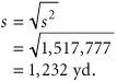
Because we haven't provided the actual data, we are also going to assume that the sample mean (  ) equals 4,200 yards and the sample standard deviation ( s ) equals 1,232 yards, although normally these values would be computed directly from the data as in the previous section.
The first step in performing the chi-square test is to determine the number of observations that should be in each frequency range, if the distribution is normal. We start by determining the area (or probability) that should be in each class, using the sample mean and standard deviation. Figure 11.14 shows the theoretical normal distribution, with the area in each range. The area of probability for each range is computed using the normal probability table (Table A.1 in Appendix A), as demonstrated earlier in this chapter. For example, the area less than 1,000 yards is determined by computing the Z statistic for x = 1,000:
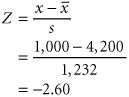
Figure 11.14. The theoretical normal distribution
(This item is displayed on page 500 in the print version)
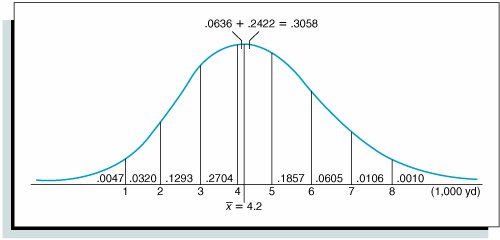
This corresponds to a normal table value of .4953. This is the area from 1,000 to the sample mean (4,200). Subtracting this value from .5000 results in the area less than 1,000, or .5000 .4953 = .0047. The area in the range of 1,000 to 2,000 yards is computed by subtracting the area from 2,000 to the mean (.4633) from the area from 1,000 to the mean (.4953), or .4953 .4633 = .0320. The Z values for these ranges and all the range areas in Figure 11.14 are shown in Table 11.2.
Table 11.2. The determination of the theoretical range frequencies
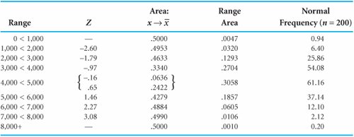
Notice that the area for the range that includes the mean between 4,000 and 5,000 yards is determined by adding the two areas to the immediate right and left of the mean, .0636 + .2422 = .3058.
The next step is to compute the theoretical frequency for each range by multiplying the area in each range by n = 200. For example, the frequency in the range from 0 to 1,000 is (.0047)(200) = 0.94, and the frequency for the range from 1,000 to 2,000 is (.0320)(200) = 6.40. These and the remaining theoretical frequencies are shown in the last column in Table 11.2.
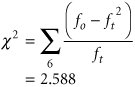
Next we must compare these theoretical frequencies with the actual frequencies in each range, using the following chi-square test statistic:
where
| f o | = | observed frequency |
| f t | = | theoretical frequency |
| k | = | the number of classes or ranges |
| p | = | the number of estimated parameters |
| k - p - 1 | = | degrees of freedom |
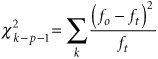
However, before we can apply this formula, we must make an important adjustment. Before we can apply the chi-square test, each range must include at least five theoretical observations. Thus, we need to combine some of the ranges so that they will contain at least five theoretical observations. For our distribution we can accomplish this by combining the two lower class ranges (01,000 and 1,0002,000) and the three higher ranges (6,0007,000; 7,0008,000; and 8,000+). This results in a revised frequency distribution with six frequency classes, as shown in Table 11.3.
Table 11.3. Computation of c 2 test statistic
| Range, Weekly Demand | Observed Frequency f o | Theoretical Frequency f t | ( f o f t ) 2 | ( f o f t ) 2 / f t |
|---|---|---|---|---|
| 0 < 2,000 | 7 | 7.34 | .12 | .016 |
| 2,000 < 3,000 | 22 | 25.86 | 14.90 | .576 |
| 3,000 < 4,000 | 50 | 54.08 | 16.64 | .308 |
| 4,000 < 5,000 | 62 | 61.16 | .71 | .012 |
| 5,000 < 6,000 | 40 | 37.14 | 8.18 | .220 |
| 6,000+ | 19 | 14.42 | 21.00 | 1.456 |
| 2.588 |
The completed chi-square test statistic is shown in the last column in Table 11.3 and is computed as follows:
Next we must compare this test statistic with a critical value obtained from the chi-square table (Table A.2) in Appendix A. The degrees of freedom for the critical value are = k p 1, where k is the number of frequency classes, or 6; and p is the number of parameters that were estimated for the distribution, which in this case is 2, the sample mean and the sample standard deviation. Thus,
| k - p - 1 | = | 6 - 2 - 1 |
| = | 3 degrees of freedom |
Using a level of significance (degree of confidence) of .05 (i.e., a = .05), from Table A.2:
c 2 .05,3 = 7.815
Because 7.815 > 2.588, we accept the hypothesis that the distribution is normal. If the c 2 value of 7.815 were less than the computed c 2 test statistic, the distribution would not be considered normal.
Statistical Analysis with Excel
QM for Windows does not have statistical program modules. Therefore, to perform statistical analysis, and specifically to compute the mean and standard deviation from sample data, we must rely on Excel. Exhibit 11.1 shows the Excel spreadsheet for our Armor Carpet Store example. The average demand for the sample data (4,200) is computed in cell C16, using the formula =AVERAGE(C4:C13) , which is also shown on the formula bar at the top of the spreadsheet. Cell C17 contains the sample standard deviation (1,231.98), computed by using the formula =STDEV(C4:C13) .
Exhibit 11.1.

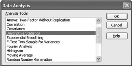
A statistical analysis of the sample data can also be obtained by using the "Data Analysis" option from the "Tools" menu at the top of the spreadsheet. (If this option is not available on your "Tools" menu, select the "Add-Ins" option from the "Tools" menu and then select the "Analysis ToolPak" option. This will insert the "Data Analysis" option on your "Tools" menu when you return to it.) Selecting the "Data Analysis" option from the "Tools" menu will result in the Data Analysis window shown in Exhibit 11.2.
Exhibit 11.2.
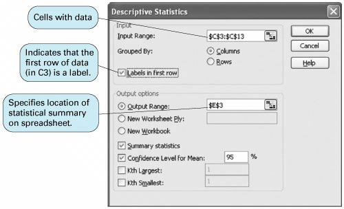
Select "Descriptive Statistics" from this window. This will result in the dialog window titled Descriptive Statistics shown in Exhibit 11.3. This window, completed as shown, results in summary statistics for the demand data in our carpet store example. Notice that the input range we entered, C3:C13 , includes the "Demand" heading on the spreadsheet in cell C3, which we acknowledge by checking the "Labels in first row" box. This will result in our statistical summary being labeled "Demand" on the spreadsheet, as shown in cell E3 in Exhibit 11.1. Notice that we indicated where we wanted to locate the summary statistics on our spreadsheet by typing E3 in the "Output Range" window. We obtained the summary statistics by checking the "Summary Statistics" box at the bottom of the screen.
Exhibit 11.3.
EAN: 2147483647
Pages: 358
- Measuring and Managing E-Business Initiatives Through the Balanced Scorecard
- A View on Knowledge Management: Utilizing a Balanced Scorecard Methodology for Analyzing Knowledge Metrics
- Measuring ROI in E-Commerce Applications: Analysis to Action
- Governance in IT Outsourcing Partnerships
- Governance Structures for IT in the Health Care Industry