Solution of Nonlinear Programming Problems with Excel | Introduction to Management Science (10th Edition)

[Page 458 ( continued )]

Excel can solve nonlinear programming problems by using the "Solver" option from the "Tools" menu that we used previously in this text to solve linear programming problems. Exhibit 10.1 shows an Excel spreadsheet set up to solve our initial Western Clothing Company example. The demand function contained in cell C4 is = 1500-24.6*C5 . The formula for profit is contained in cell C3 and is shown on the formula bar at the top of the spreadsheet.

Exhibit 10.1.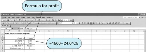

The Solver Parameters window for this problem is shown in Exhibit 10.2. It is important to check the "Options" settings from Solver and make sure that the "Assume Linear Models" option has not been selected. Solver will automatically solve the problem as a nonlinear model if the "Assume Linear Model" option has not been selected. Exhibit 10.3 shows the Excel solution for the Western Clothing Company example.

Exhibit 10.2.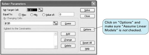

[Page 459]

Exhibit 10.3.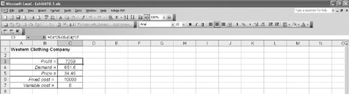

Exhibit 10.4 shows an Excel spreadsheet set up to solve a nonlinear version of the Beaver Creek Pottery Company example from Chapter 2 that is formulated as

maximize Z = $(4 0.1 x ₁ ) x ₁ + (5 0.2 x ₂ ) x ₂

subject to

x ₁ + 2 x ₂ = 40 hours (labor)

where

x ₁	=	number of bowls produced
x ₂	=	number of mugs produced
4 0.1 x ₁	=	profit ($) per bowl
5 0.2 x ₂	=	profit ($) per mug

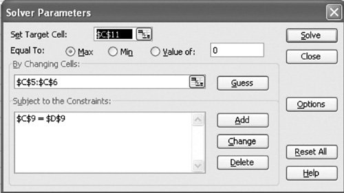
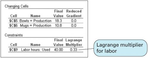
Exhibit 10.4.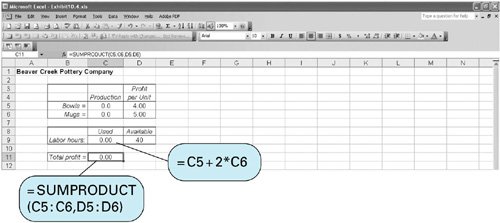

The numbers of bowls and mugs produced are contained in cells C5 and C6, respectively. The profit formula for a bowl is contained in cell D5. The total profit contained in cell C11 is computed using the formula =SUMPRODUCT ( C5:C6,D5:D6 ) and is shown on the formula bar at the top of the spreadsheet. The formula for labor, =C5+2*C6 , is contained in cell C9. The Solver Parameters window for this problem is shown in Exhibit 10.5, and the final solution is shown in Exhibit 10.6.

Exhibit 10.5.

(This item is displayed on page 460 in the print version)

Exhibit 10.6.

(This item is displayed on page 460 in the print version)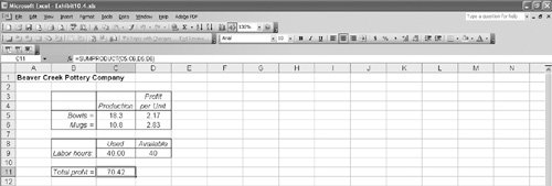

Excel will also provide the value of the Lagrange multiplier , which provides the dual value of the labor resource. To derive the Lagrange multiplier, after you click on "Solve" in Solver, the Solver Results screen shown in Exhibit 10.7 will appear. On this screen, under "Reports," select "Sensitivity." This will generate the sensitivity report shown in Exhibit 10.8. Note that in addition to the problem solution, the value of the Lagrange multiplier is also provided for the labor constraint.

[Page 460]

Exhibit 10.7.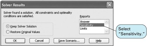

Exhibit 10.8.

The Lagrange multiplier value of .33 is analogous to the dual value in a linear programming problem. It reflects the approximate change in the objective function resulting from a unit change in the quantity (right-hand-side) value of the constraint equation. For this example, if the quantity of labor hours is increased from 40 to 41 hours, the value of Z will increase by $0.33from $70.42 to $70.75.