Section 6.3. DATA

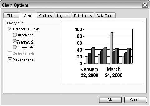
6.2. CREATING AND FORMATTING CHARTS

6.2.1. Use Dates on the X-Axis

THE ANNOYANCE: I want the X-axis of my chart to be a bunch of dates. What do I do?

THE FIX: Right-click the X-axis and choose Format Axis. Click the Number tab, and choose Date in the Category list (see Figure 6-10). If you don't see the date style you want in the Type list, choose Custom in the Category list and create what you need. For example, to display your dates as Friday, August 30, 2002, select Custom and input dddd, mmmm d, yyyy in the Type area.

Figure 6-10. To specify the settings for numbers on your chart, choose from a variety of categories on the left: percentages, time, date, number (where you can set the number of decimal points), etc., and make category-specific adjustments on the right.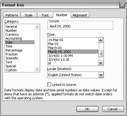

If, for some reason, the date in your chart does not show up properly even after you've selected the date format on the Number tab, select Chart Chart Options, click the Axes tab, and choose the Category or Time-scale option under Category (X) axis (see Figure 6-11).

Figure 6-11. Occasionally your axis won't behave correctly even after you've formatted the numbers. In that case, select Chart Chart Options and choose either the Category or Time-scale option on the Axes tab.

6.2.2. Create a Combination Chart

THE ANNOYANCE: I need to make a combination column and line chart. That is, I need to have a column chart, but I want one of the data series to be a line. I can't find this kind of chart in the available choices. Did I just miss it?

THE FIX: To create a combination column-line chart in PowerPoint, create a column chart using all your data series. Right-click the "line" series and choose Chart Type (see Figure 6-12). Select a line chart from the dialog box, make sure the "Apply to selection" box is checked, and click OK; the data series will become a line (see Figure 6-13).

Figure 6-12. To create a combination column-line chart, right-click a column data series, choose Chart Type, and select a line chart type from the list on the left.

Figure 6-13. The selected data series is now a line.

The possible combinations depend on the types of charts with which you're working. For example, you can't combine many 3D charts with each other, and you also can't combine 2D and 3D charts.

6.2.3. Create a Secondary Axis

THE ANNOYANCE: I have a bunch of wildly disparate data I'd like to plot on two different axes, but I can't figure out how to add another axis and tie some of the data to it.

THE FIX: Right-click a data series, choose Format Data Series, click the Axis tab, and choose the Secondary axis option (see Figure 6-14). Repeat for any other data series you want to tie to the secondary axis.

Figure 6-14. Choose the Secondary axis option to plot data on a secondary axis.

6.2.4. Add Error Bars to Data Points

THE ANNOYANCE: I need to add error bars to all the points on my data series, but the values are different for each point. Do I have to draw these in manually? This will not only be incredibly tedious, but also very inaccurate. Is there a better way?

THE FIX: You can either create your chart in Excel, where you can input a range of values for your error bars, or you can use the Stock chart type in PowerPoint. It's best to use Excel for these charts, as Excel offers much more flexibility than the Stock chart type in PowerPoint.

To add error bars in Excel, create your chart, right-click a data series, and choose Format Data Series. On the Y Error Bars tab, click the "Custom +" button (see Figure 6-15). Click and drag on the spreadsheet to select the range of data representing the positive side of the error bars for the seriesthe data will be added to the "Custom +" area of the dialog box. Click the button on the right (see Figure 6-16) to expand the dialog box and repeat the process for the "Custom" values. If the positive and negative error bar values are the same, you can input the same data range.

Figure 6-15. In Excel, you can add a range of values for custom error bars. PowerPoint does not have this option. Simply click the button to the right of "Custom +" or "Custom -" to add values for the error bars.

Figure 6-16. After you click the button on the Y Error Bar tab to collapse the dialog box so you can select data, your screen will look something like this. Click and drag across the data range on the spreadsheet; it will be added automatically to the custom range area. Click the Select button to expand the dialog box.

To format the error bars, right-click one (which selects all error bars in the series) and choose Format Error Bars. Change the marker, line weight, color, and style on the Patterns tab.

To manipulate the Stock chart type in PowerPoint to display error bars, use the following steps:

Create a chart based on the Stock Chart Type.
Select Insert Chart, and with the chart activated, choose Chart Chart Type, choose Stock (High-Low-Close) from the list, and click OK (see Figure 6-17). You will start with this chart based on PowerPoints default dummy data.
Select View Datasheet and change the dummy data to your actual data. East represents the high point of the error bar, West represents the low point of the error bar, and North represents the data point itself (see Figure 6-18).

Figure 6-17. Start with a Stock chart to add individual error bars in PowerPoint.

Figure 6-18. Replace dummy data with your own data. In a High-Low-Close Stock chart, the first data series represents the top point of the high-low lines, and the second data series represents the bottom point. The third data series is the actual data point.
Format the North (Data) points into columns.
Right-click the little dash representing the North (Data) series and choose Chart Type. Select Column from the Chart Type list, make sure the "Apply to selection" box is checked, and click OK (see Figure 6-12).
Format the error bars.
Right-click one of the high-low lines, choose Format High-Low lines, and change the line style, weight, and color as desired. Note that high-low lines don't have the "T" caps. If you need your error bars to have caps, you'll need to create the chart in Excel.

6.2.5. Create an Axis Break

THE ANNOYANCE: I can't add a break to the Y-axis labels. Since the values of my data are so different, I need to show 0 to 25, a break, and then 80 to 100. Any suggestions?

THE FIX: Honestly, it's easiest to just draw a couple of hash marks to represent a break on the Y-axis. You can add AutoShapes to create breaks for the columns, too, if you wish.

Neither Excel nor PowerPoint includes a "break-axis" option, although Microsoft Excel MVPs Tushar Mehta (http://www.tushar-mehta.com/excel/newsgroups/broken_y_axis/tutorial/index.html), Jon Peltier (http://peltiertech.com/Excel/Charts/BrokenYAxis.html), and Andy Pope (http://www.andypope.info/charts/brokencolumn.htm) have all posted techniques for displaying broken axes.

Use the following steps to create a chart with a broken Y-axis in PowerPoint:

Make a copy of your chart.
Because this technique requires changing the data in your datasheet, you'll want to keep a copy of your actual chart in case you need to revisit the data later. Select the chart on the slide, press Ctrl+C to copy it, and press Ctrl+V to paste it. Right-click the copy, choose Format Object, click the Size tab, and set the scale to 5%x5%. Drag this off the edge of the slide where it won't show during a presentation.
Change the data.
Change the uppermost data value so it's closer to the smaller data values. You'll replace the upper Y-axis numbers later (see Figure 6-19). Select View Datasheet to open the datasheet if its not already open.
Change the axis scale.
Right-click the Y axis, choose Format Axis, click the Scale tab, and change the maximum value to something lower than it was, but still high enough to exceed your largest data point (see Figure 6-20).

Figure 6-19. The original data and chart is shown in the top screenshot. In the bottom screenshot, we subtracted 40 from each of the large data points to make them closer to the smaller data point.

Figure 6-20. After changing the data, the largest point is 56. Thus, 60 is a good point to use for the Y-axis scale maximum.
Draw the axis break.
Click the slide to deactivate the chart, select AutoShapes Basic Shapes Parallelogram, and draw a parallelogram on the slide. Size and rotate it appropriately along the Y-axis. Draw a line on the top edge of the parallelogram, copy it, and position it at the bottom edge of the parallelogram (see Figure 6-21).

Figure 6-21. A parallelogram and two lines make up the axis break. If you plan to print the chart, check the black and white settings to make sure the "break" objects will print the way you want.

Double-click the parallelogram, and on the Colors and Lines tab, choose Background from the Color drop-down menu in the Fill area. Next, choose No Line from the Color drop-down menu in the Line area and click OK to exit the dialog. Select the parallelogram and the two lines and choose Draw Group to group the three items.
Align or Distribute Align Right to align the labels (see Figure 6-22).

Figure 6-22. Add new Y-axis values in text boxes on the slide. Press the arrows on your keyboard to nudge them, and choose Draw Align or Distribute to align them.
Remove existing Y-axis labels.
Right-click the chart and choose Chart Object Edit to activate it. Click the Y-axis, choose Format Selected Axis, and click the Patterns tab. Remove the Y-axis labels by selecting None in the "Tick mark labels section (see Figure 6-23).

Figure 6-23. You can remove tick marks and axis labels from an axis.
Make final adjustments.
Click outside the chart to deactivate it. If you wish, add parallelograms to "break" the tall columns (see Figure 6-24). Adjust the placement of the axis-label text boxes and axis break lines as necessary.

Figure 6-24. This is the final chart showing the axis break. Parallelograms were also added on top of the columns to more clearly represent the break in the data.

Get Rid of Chart Junk

As much as Edward Tufte frustrates me with his whole "Cognitive Style of PowerPoint" invective, he's still the godfather of displaying data. Take his advice and eliminate the extraneous clutter on your charts wherever you can: tick marks, axis labels coupled with data point labels, unreadable fonts, etc. And include a reference for the data on the slide.

6.2.6. Remove Percent Markers from Y-Axis

THE ANNOYANCE: Our corporate style specifies that we use the word "Percent" in the Y-axis title and not put "%" on the Y-axis label numbers. That's fine, but all the charts I receive are already plotted as percentages. Is there an easy way around this?

THE FIX: There's no perfect way around this issue. The best way is probably to copy the data into Excel, multiply by 100, and paste it back into the PowerPoint datasheet. Of course, you must select Format Number to change the datas number format to "number" or "general" instead of "percentage."

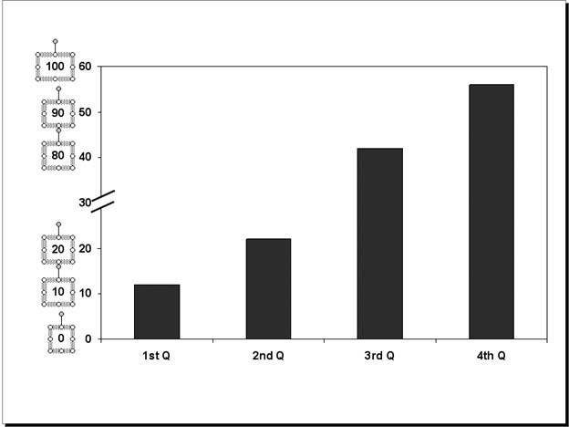
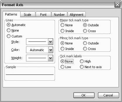
You can also remove the Y-axis labels. Select Format Selected Axis, click the Patterns tab, choose None in the "Tick mark labels section (see Figure 6-23), and then add text boxes with just the numbers.

Or you can draw a rectangle to cover the existing axis labels, select Format AutoShape, click the Colors and Lines tab, and choose Background from the Color drop-down menu. Next, choose No Line from the Color drop-down menu in the Line area to make the cover blend into the background. Finally, add text boxes with the new axis labels.

6.2.7. Add Percent Markers to the Y-Axis

THE ANNOYANCE: Can I add a % symbol to the Y-axis labels without having to redo all the data? My chart looks almost exactly the way I want it to right now, and I'd really rather not have to reformat it.

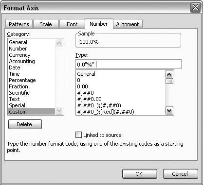
THE FIX: Activate the chart, right-click the Y-axis and choose Format Axis. Click the Number tab, choose Custom from the Category list, and enter 0.0"%" in the Type box. The quotation marks tell MSGraph to add the percent sign as a text character without replotting the values as percents (see Figure 6-25).

Figure 6-25. You can add text to the numbers on your value axis by enclosing the text in quotation marks.

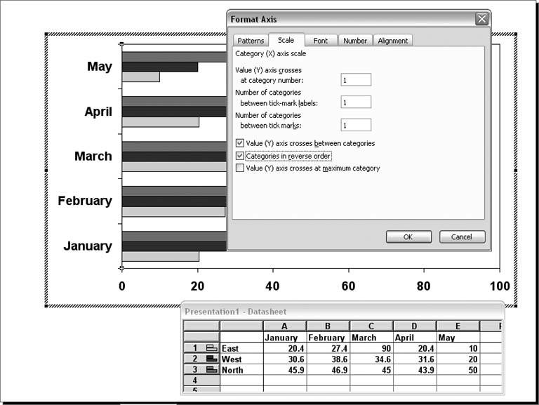
6.2.8. Reverse Order of Categories

THE ANNOYANCE: My chart is plotted backward! How can I change the order?

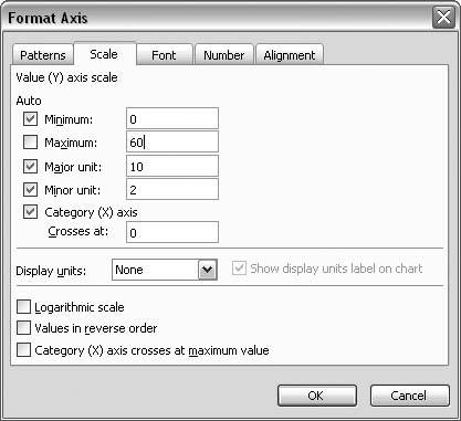
THE FIX: Activate the chart, select the category axis, choose Format Selected Axis, click the Scale tab, and check the "Categories in reverse order box (see Figure 6-26).

Figure 6-26. Check the "Categories in reverse order" box to reverse the plot order of categories.

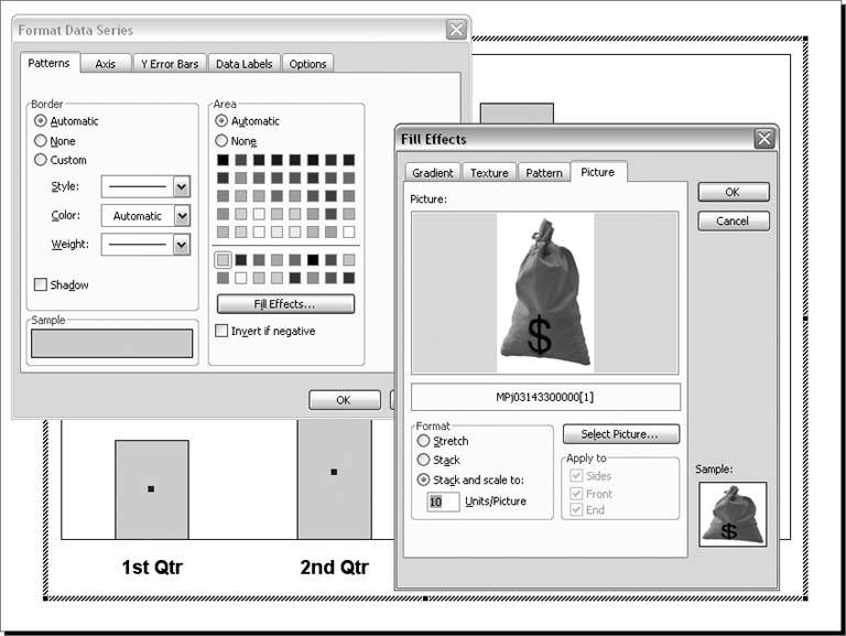
6.2.9. Insert Picture Fills

THE ANNOYANCE: Can I use a picture or clip art for my data points?

THE FIX: Sure! Select your data series, choose Format Selected Data Series, click the Patterns tab, click the Fill Effects button, and click the Picture tab. Select an appropriate picture, check the settings you want (see Figure 6-27), and click OK.

Figure 6-27. In addition to the familiar solid colors, you can fill chart data points with pictures, patterns, gradients, and textures.

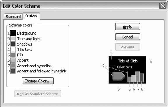
6.2.10. Change Chart Colors

THE ANNOYANCE: I don't like the colors on the chart in this template. How can I change the colors so I don't have to hand-format every single one?

THE FIX: The colors in a chart are actually tied directly to the slide color scheme. To change the colors in the chart, you must change the colors in the slide color scheme.

In PowerPoint 2002 and 2003, select Format Slide Design, click Color Schemes in the task pane, and then click Edit Color Schemes at the bottom of the task pane. In PowerPoint 97 and 2000, select Format Slide Color Scheme and click the Custom tab. The first data series will take the color assigned to "Fills," the second series will use "Accent," the third will use "Accent and hyperlink," and the fourth, "Accent and followed hyperlink (see Figure 6-28).

Figure 6-28. The slide color scheme governs the colors of data in charts.

Or create your charts in Excel. Select Tools Options, click the Color tab, and then click the Modify button to change any of the colors in any of the available swatches. Next, select File Save and save the worksheet to your hard drive. You can then use it as a color master. Open another Excel workbook, create your chart, choose Tools Options, click the Color tab, and choose the color master file from the "Copy colors from drop-down menu. The menu lists only open Excel files, so make sure your color master file is open when you're ready to copy colors into a new file.

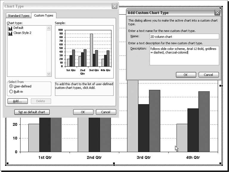
6.2.11. Create a Default Chart

THE ANNOYANCE: Every single time I create a chart, I have to change the chart type from that stupid 3D column chart. Can I use a different chart type as the default?

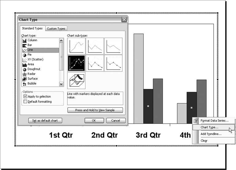
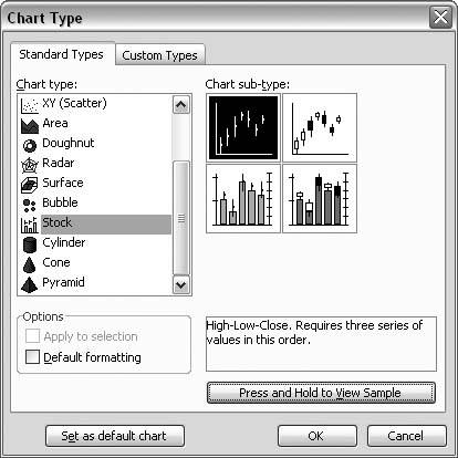
THE FIX: Absolutely! Go find or create a chart you want as your default, choose Chart Chart Type, click the Custom Types tab, choose the User-defined option, and click the "Set as default chart button. When asked if you're sure, click Yes, and then fill in the dialog box to add the chart to the list of user-defined charts (see Figure 6-29).

Figure 6-29. Click the "Set as default chart" button to set a default chart style. Unfortunately, these user-defined and default charts are specific to a computer, not to a presentation or template file.

If you would just like to add a chart style to your arsenal to save some formatting time, simply click the Add button. This adds the chart to your user-defined chart style list, but it does not replace the default chart style. When you create default and user-defined charts, you should be aware of the following:

If your default chart follows your slide color scheme, when you create a new chart on a slide with a different color scheme, the chart will follow the new slide's color scheme.
User-defined charts are machine-specific settings. That means these chart styles do not travel with the template or the presentation.
The file GRUSRGAL.GRA contains your user-defined and default chart settings. If you want to try replacing another user's GRUSRGAL.GRA file with your own, you can usually find this file in the following folder: C:\Documents and Settings\[UserName]\Application Data\Microsoft\Graph. Replacing someone's GRUSRGAL.GRA file will delete any user-defined chart styles he may have created.
You cannot globally change the fill color swatches on the Patterns tab (see Figure 6-30). You can, however, modify these swatches (select Tools Options, click the Color tab, and click the Modify button) for an Figure 6-30. The colors you see on the Patterns tab reset to these default colors each time you create a new chart. However, the colors indicated do change according to the slide color scheme.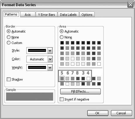
If you need more colors for your charts, modify the 40 fill color swatches. Select Tools Options, click the Color tab, and click the Modify button. Next, create a chart using those colors and include it on a slide. Instruct your users to paste that slide and change the data in the chart to create more charts.

6.2.12. Reset the Default Chart Style

THE ANNOYANCE: I tried to create a new default graph style, but I messed up. How do I get the old default chart back?

THE FIX: Just delete the current default chart type and it will reset to the original. Select Chart Chart Type, choose the User-defined option, choose Default from the list, and click the Delete button.

6.2.13. Charts Recolor When Pasted into Presentations

THE ANNOYANCE: When I paste my chart into a different presentation, it changes colors.

THE FIX: Before you paste the slide or chart into the new presentation, select it and choose View Toolbars Picture. Click the Recolor Chart button and choose None from the options (see Figure 6-31). You may want to experiment with selecting the recolor "only text and background option as well (see Figure 6-32).

Figure 6-31. Click the Recolor Chart button on the Picture toolbar to specify what happens to the chart colors when you paste the chart onto a slide using a different color scheme.

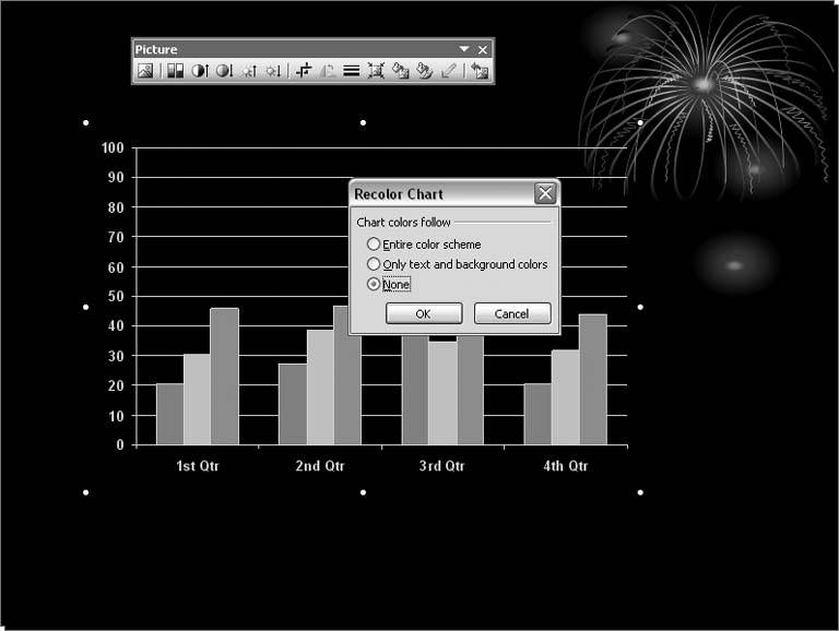
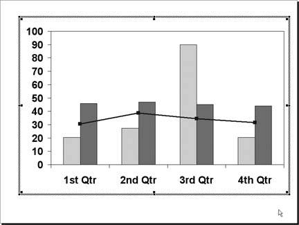
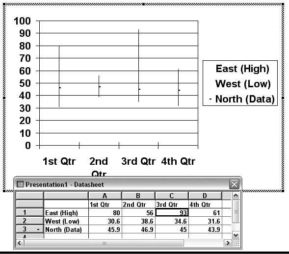
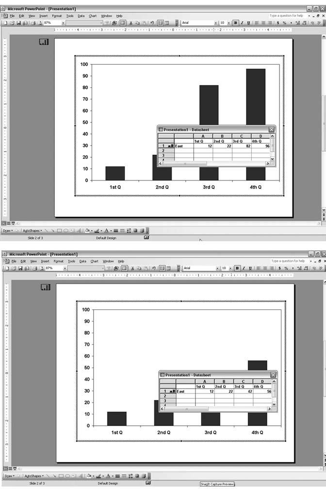
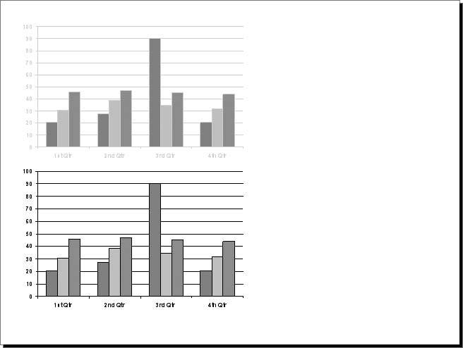
Figure 6-32. The top chart shows what happens when you paste the chart after choosing None in the Recolor Chart options. The chart on the bottom shows the results of choosing to recolor "only text and background."

Alternatively, you can select the chart after you've pasted it into the new presentation and choose the Recolor Chart button on the Picture toolbar. This technique also works well on Excel charts imported into PowerPoint, and is a fantastic way to leverage Excel's color management (in Excel, choose Tools Options, click the Color tab, and make a selection from the "Copy colors from drop-down list) on charts in PowerPoint.

6.2.14. Change Settings for Printing in Black and White

THE ANNOYANCE: I have a chart with a bunch of data points, and I can't tell them apart when I print to a black and white printerall the different shades of gray are too close. What should I do?

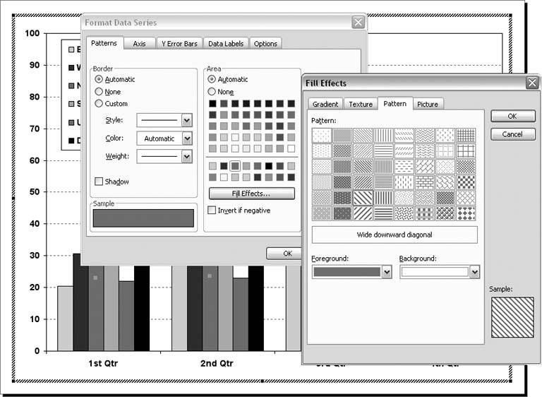
THE FIX: Specify pattern fills for some of the data points or series. Right-click a data series, choose Format Data Series, click the Patterns tab, click the Fill Effects button, and click the Pattern tab (see Figure 6-33). For maximum contrast, choose black for the Foreground and white for the Background colors. Of course, do this type of thing on a copy of the slide or presentation so you don't mess up the colors on the real presentation files. You may also need to change the actual color of some of the data points to black, white, medium gray, and light gray.

Figure 6-33. Adding a pattern fill to a data point or data series makes it easy to identify in black-and-white prints.

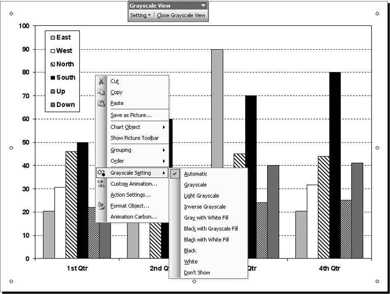
Don't forget to check the Black and White settings for the chart. Click the slide to deactivate the chart and select View Color/Grayscale Grayscale or Pure Black and White. (In PowerPoint 97 and 2000, select View Black and White.) Next, right-click the chart, select the Grayscale or Black and White setting, and choose another option from the list (see Figure 6-34).

Figure 6-34. Black and White or Grayscale settings also have some bearing on how a chart looks when printed in black and white. Unfortunately these settings apply to the chart as a whole and cannot be applied to the individual elements of the chart.

6.2.15. Charts Appear Flipped

THE ANNOYANCE: My office upgraded to PowerPoint 2002, but when I view the charts I created in PowerPoint 2000, they appear flipped. Do we have to downgrade to 2000?

THE FIX: Open the file in PowerPoint 97 or 2000, select the chart, choose Draw Rotate or Flip to rotate it appropriately, and save the presentation.

Unfortunately, you can't reset charts to their original orientation in PowerPoint 2002 or 2003.

6.2.16. Charts Resize When Opened

THE ANNOYANCE: When I double-click my chart and open it, it's not the same size as on the slide.

THE FIX: This is because you dragged the edges of the chart when you were looking at it on the slide. And you didn't drag the edges proportionately (that is, drag the corner). To fix it, close the chart, right-click it, choose Format Object, click the Size tab, specify 100% in the Scale area, and click OK. Then double-click to open and resize the chart by dragging the "herringbone edges (see Figure 6-4 earlier in this chapter).

Resize a chart only when it is activated. If you must resize a chart when it's not activated, maintain its aspect ratio by dragging a corner.

Other Charting Options

If compatibility is not a huge issue for you, there are a number of charting programs available aside from Excel and PowerPoint's Microsoft Graph. Some do extensive statistical functions and analysis, others are best at making pretty charts from the data. Most of the heavy-duty statistical programs will at least export images, which you can then insert into PowerPoint. Others will insert into slides as OLE linked or embedded objects. Some even convert graphs to Flash and other formats, which often allows for sophisticated animations.

PowerPlugs: Charts (http://www.crystalgraphics.com/presentations/charts.main.asp) costs $99.
MekkoGraphics (http://www.mekkographics.com/) Basic Edition costs $99 and the Professional Edition costs $499.
Swiff Chart (http://www.globfx.com/products/swfchart/) costs $149.
XcelsiusXL (http://www.infommersion.com/index.html) costs $195 for the Standard version and $495 for the Professional version.
KaleidaGraph (http://www.synergy.com/) costs $200 but the company offers a discount for academic institutions.
Delta Graph (http://www.rockware.com/catalog/pages/deltagraphw.html) costs $295, but the company offers a discount for academic institutions.
Grapher (http://www.goldensoftware.com/products/grapher/grapher.shtml) costs $299.
Prism (http://www.graphpad.com/prism/Prism.htm) costs $371.25 for qualified students, $495 for commercial enterprises, and $445 for academic institutions.
Miner3D (http://miner3d.com/index.html) Basic Edition costs $495 and the Professional Edition costs $875.
Adobe Illustrator (http://www.adobe.com/products/illustrator/main.html) costs $499.
SigmaPlot (http://www.systat.com/products/) costs $499 for academic institutions, $579 for government organizations, and $699 for commercial enterprises.
Origin Lab (http://www.originlab.com/) is available to individuals and academic, government, and commercial clients. Check its web site for prices.
S-Plus (http://www.insightful.com/products/splus/default.asp). Email a company sales person for a price quote.
SPSS Base (http://www.spss.com/) costs $1,599
While not a true graphing program, Perspector (http://www.perspector.com/) is a fantastic 3D business graphics creator for PowerPoint. The Standard version costs $69 and the Professional version costs $199.