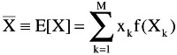
|
Six Sigma and Beyond. Statistics and Probability Authors: Stamatis D.H. Published year: 2003 Pages: 198-199/252 |
MEAN from RV Range: M discrete values or cells , X k
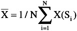
or MEAN from Sample Space: N discrete individual samples, S i
Sum produced by pair of fair six-sided dice.
Random Variable X k defined as sum of the two numbers :
X k = {D 1 + D 2 }
|
Cell k |
No. in X k |
X k |
f (X k ) |
X k f (X k ) |
|---|---|---|---|---|
|
1 |
1 |
2 |
1/36 |
2/36 |
|
2 |
2 |
3 |
2/36 |
6/36 |
|
3 |
3 |
4 |
3/36 |
12/36 |
|
4 |
4 |
5 |
4/36 |
20/36 |
|
5 |
5 |
6 |
5/36 |
30/36 |
|
6 |
6 |
7 |
6/36 |
42/36 |
|
7 |
5 |
8 |
5/36 |
40/36 |
|
8 |
4 |
9 |
4/36 |
36/36 |
|
9 |
3 |
10 |
3/36 |
30/36 |
|
10 |
2 |
11 |
2/36 |
22/36 |
|
11 |
1 |
12 |
1/36 |
12/36 |
|
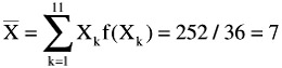
M = 11 |
36 |
Sum 252/36 |
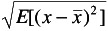
Sample variance and standard deviation
Sample variance: Expected value of X i about the mean
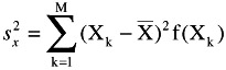
or
Sample standard deviation: s
x
‰
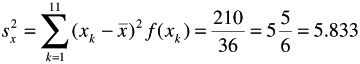
Exercise: Sum of two fair dice: X k = {D 1 + D 2 }
|
x k |
(X
k
-
|
(X
k
-
|
f(X k ) |
(X
k
-
|
|---|---|---|---|---|
|
2 |
-5 |
25 |
1/36 |
25/36 |
|
3 |
-4 |
16 |
2/36 |
32/36 |
|
4 |
-3 |
9 |
3/36 |
27/36 |
|
5 |
-2 |
4 |
4/36 |
16/36 |
|
6 |
-1 |
1 |
5/36 |
5/36 |
|
7 |
6/36 |
|||
|
8 |
1 |
1 |
5/36 |
5/36 |
|
9 |
2 |
4 |
4/36 |
16/36 |
|
10 |
3 |
9 |
3/36 |
27/36 |
|
11 |
4 |
16 |
2/36 |
32/36 |
|
12 |
5 |
25 |
1/36 |
25/36 |
|
Sum 210/36 |
Variance:
Standard deviation:
s x = 2.415
As we have mentioned earlier, discrete random variables are represented by isolated real-valued numbers . Manipulation of discrete random variables involves summations of these discrete values. This is illustrated for the frequency of outcomes in k- cells ; n = total number samples.
Probability density function (pdf): f(X
k
) =
Cumulative distribution function (CDF) (sum)
Mean
Variance
Integrals (areas) of continuous r.v. x yield closed form equations that are easy to manipulate and to analyze.
Integrals of standardized distributions can be tabulated.
Probability density function (pdf): f (x) where probabilities are only defined as the area within an interval.
Two constraints of a probability density function: f (x)
Positive value: f(x)
Unit area:
f
(
x
)
dx
1
Cumulative distribution function (CDF): F(x) = (
P
(-
ˆ
<
X
x
) =
f
(
x
)
dx
f(x) = dF(x)/dx
These functions may be represented by the graphs in Figure 16.6.
Figure 16.6:
The probability (left) and cumulative (right) functions.
Probability is defined only in the context of an incremental range of the random variable [a x b].
Probabilities cannot be determined for a point x , since the interval of integration or the base (b - a) is zero.
Probabilities can be determined from either the probability density function f(x) or the cumulative distribution function F(x).
The CDF is more important because tabulated values of the various standardized or normalized probability distributions models presented in this form.
Mean:
Variance:
|
Six Sigma and Beyond. Statistics and Probability Authors: Stamatis D.H. Published year: 2003 Pages: 198-199/252 |