AN SPC APPLICATION FOR STATISTICAL INVENTORY CONTROL

In this explanation of statistical inventory control, I will represent mathematical formulas using the latest notation as much as possible. Stochastic (random) variables will be denoted by lower case (e.g., x or d ) underlined . A stochastic variable is one whose value is entirely a matter of chance.

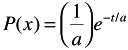
If a stochastic variable x can only assume discrete values (e.g., the number of orders per week), then P ( x ) = P { x = x} is the probability that the variable x will assume a specific value x.

Since the number of possible values of x _i is infinite in theory and the sum of all the probability must be unity, we have

The stochastic variable x then has a discrete or discontinous probability distribution.

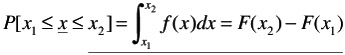
The "distribution fraction" of x is given by F ( x ) = P ( x x ). On the other hand, for a discontinous probability distribution, the distribution function is, of course, a step function.

The continous probability distribution is probability distribution in which the variable continously can assume any of the values throughout a given range, while F ( x ) is continuous and differentiable for all these values.

The density function ( x ) of the distribution is defined by

Now we have

and

The mathematical probability E ( ( x )) of a function of a stochastic variable is defined by

for a discrete probability distribution, and by

for a continuous distribution. The following are special cases:

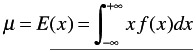
1. The mean value of x itself (denoted by ¼ )

   

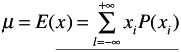
   and

   

2. The variance ƒ ² of x . This is deduced from

   (17.1)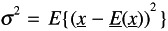 

   

For a discrete probability distribution, then, we have

For a continuous probability distribution

An alternative expression for Equation 17.1 exists and is derived as follows :

ƒ ² = E ( x ² )-( E ( x )) ²

E ( x ² )= ƒ ² +( E ( x )) ²

SOME THEORETICAL DISTRIBUTIONS

Exponential

If one considers the distribution density of the interval t between two consecutive events in circumstances identical with those in which the number of events per time unit follows a Poisson distribution:

P ( o ) = e ^{- ¼}

The probability that no event will take place in t consecutive periods is equivalent to

( e ^{- ¼} ) t = e ^{- ¼ t}

The probability that the interval t is between the values t and t + dt is equal to the probability that no event will take place during t time units, multiplied by the probability that an event will occur in the subsequent short time span dt. Formulated:

(17.2) 

This distribution, which is continuous, is called the (negative) exponential distribution. From the equations of ¼ and ƒ ² and by means of partial integration, we can readily ascertain that for this distribution

and

Accordingly, an exponential distribution with mean and standard deviation a can be formulated as follows:

From Equation 17.2 we can readily establish the distribution function F ( t ) as follows:

Therefore

p ( t > t )= e ^{- ¼ t}

THE GAMMA DISTRIBUTION

A theoretical distribution having many uses in studies of writing times and stock (inventories) is what is known as the gamma distribution. This is a single-peaked, continuous-frequency distribution, whose coefficient of variation can be varied between 1 and 0. Moreover, this distribution lends itself well to mathematical treatment.

For this example I will employ only those gamma distributions whose starting points are at 0. The general form of these distributions is as follows:

(17.3)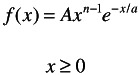 

where a is the scale parameter governing the mean value for a given form. The parameter n is called the form parameter and governs the shape of the curve. For integral values of n, A (Equation 17.4) takes the form

(17.4)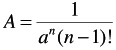 

The gamma distribution may be regarded as the distribution of the sum of n independent values drawn at random from an integral exponential distribution having a mean a. For example, from Equations 17.3 and 17.4 a gamma distribution with a=2 is

f ( x ) = ¼ ² xe ^{- ¼ x} , x

It can be also shown that the sum of two quantities following gamma distribution, having the same scale parameter a but with form parameters n ₁ and n ₂ , follows a gamma distribution with a scale parameter a and a form parameter ( n ₁ + n ₂ ). Other equations applicable to the gamma distribution are E ( x ) = an and

ƒ ² = E { x - E ( x )} ² = na ²

It is often convenient to determine the chances of excess for the gamma distribution by making use of the relationship between this and the x ² distribution. The reason is that x ² = 2 x / ± is found to follow an x ² having 2 n degrees of freedom, if x follows a gamma distribution with parameters a and n.

If the mean Xbar and standard deviations s of these observations have been calculated, then the simplest way to adapt a gamma distribution is as follows:

Calculate n from

and then a from

It is of importance to note that toward higher values of n, a normal distribution provides a better approximation of the gamma distribution; for the purpose of an inventory control problem, a sufficiently close approximation is usually obtained above n = 20; a different limit of n = 50 is required only for the tail of the distribution (probabilities of error 1% and lower).

SPECIAL APPLICATIONS AND FORMULAS FOR SOLVING INVENTORY PROBLEMS

Case 1. One Stock Point: Demand Known and Constant

Assumptions:

• The entire quantity Q enters the system.

• The storage space is unlimited.

• There is no discount.

• There is no need for rounding on account of life of foods etc.

• There are these kinds of variable costs:

  1. The costs of rounding, or reordering , involving an amount F on each occasion.

  2. The costs of maintaining the inventory, an amount c _i per item.

  3. The costs of stockout, representing an amount N per year and per product. A negative stock (or lag in delivery) of one product persisting throughout a whole year costs an amount of N.

  4. There is a specific demand D.

Another assumption is that cumulative lag in the deliveries is brought up to date as soon as the new replenishment quantity Q arrives. Thus the inventory becomes a quality that may be either positive or negative.

The inventory is positive for part of the time. This period is represented by ED/EC (see Figure 17.1):

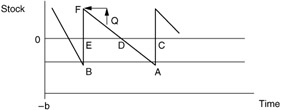
Figure 17.1: Inventory variation, constant demand.

where Q is batch quantity and b is the buffer stock.

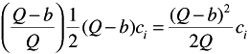
The average inventory during the time that this is positive is EF or ( Q - b ). Accordingly, the annual costs of maintaining stock are

The stock is negative during a part of the year equivalent to DC/EC so that the costs become

The total variable costs per year are then found to be

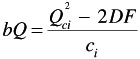
By differentiating with respect to Q or b and taking the differential quotients to be zero, we obtain, after a certain amount of simplification,

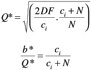
(17.5) 

(17.6) 

(17.7)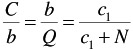 

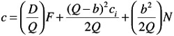
If we substitute b ( c _I + N ) = c _I Q (according to Equation 17.6 in Equation 17.5 procedures, where C = capital),

By multiplying this result for bQ by Q/b = c _i + N/c _i we obtain

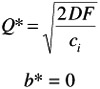
* denotes Camp's formulation of optimum batch size ; if N = ˆ then

Note 

We can also use the tool wear approach of SPC to calculate the optimum inventory cycle.